Basics

Phase spacing

1. One- and two-particle phase space
   
2. Three and more particles
   
3. MC Integration: Sampling
   

   BASIC IDEA

   In the previous sections, higher dimensional phase space integrals for processes with n outgoing particles have been evaluated analytically. However, in so doing, the effect of amplitudes squared has been totally neglected (implicitly it was set to 1, to phrase it differently). In practical applications, this function of the four-momenta of course has to be included into the integration, rendering it a difficult task. In fact, in many practical cases, especially if n becomes larger than three or if non-trivial cuts on the phase space have to be taken into account, an analytical solution for the integral is impossible and numerical methods have to be applied. Due to the high dimensionality of the phase space standard textbook methods such as simple quadratures become prohibitively time consuming and different methods suitable for high-dimensional integration have to be devised. One of these methods is called Monte-Carlo integration. The basic idea here is the following:
   Take a statistically significant sample of the function, by evaluating it at a large number of points. The average of this sample provides an estimator <I> of the function. Writing the phase space volume as an n-dimensional hypercube with dimension 1, this amounts to replacing where the various R denote n-dimensional vectors of uniformly distributed random numbers in [0,1]. It should be clear at this point that any integration of a function g(q) over the variable q in some interval [a,b] can be mapped onto an integration of a function f(x) over a variable x in [0,1]. In such a case, however, the function f contains g with q expressed through x and a corresponding Jacobian. This obviously also holds true for vectors q and x. To exemplify this, consider the two-body phase space integral where clearly the substitution has been performed.
   
   

   TRUE VALUE, ESTIMATED VALUE, CONFIDENCE AND CONVERGENCE

   In principle, in the limit of N going to infinity the estimated value <I> of the integral should approach its true value I. This limit, however, can not be reached in practise. Therefore, it is a priori not clear, how good the estimate describes reality. In fact, during numerical integration, i.e. during the sampling, <I> will in all practical cases fluctuate.
   Sometimes, these fluctuations will be severe oscillations with large factors between estimators taken after different numbers N of sampling points. This is especially true, if the integrand (the function) itself is a wildly fluctuating function, spanning orders of magnitude, maybe, to make things even worse, with extremely sharp peaks. Such peaks can clearly be missed quite easily for a long time while sampling, in the very moment one or more of them contribute to the result, the corresponding estimator will change accordingly. Examples for such fluctuating function that occur frequently in the evaluation of cross sections are connected to "propagator terms" and have the form where s is some invariant mass to be integrated over. This will be better understood once Feynman diagram techniques have been discussed. Anyways, it is obvious that, when integrating over s, the former of the two functions above diverges for s→ 0 and the latter has a Breit-Wigner-like peak for s→ M². In such cases, depending on available phase space, a sampling over s may for quite some time be quite stable, because the peak has been missed; in the two dangerous limits, however, the sum over the different sampling points may easily explode.
   Now it is time to employ a measure from statistics to judge the size of the fluctuations relative to the average, namely the variance. In so doing, some implicit assumptions have been made: first of all, it is assumed that the sample, i.e. N, is large enough to render statistical methods a valid way; second, the sampling points have been taken independently from each other. Then the variance is a good way to estimate the error range of the estimator. To employ this concept in such Monte-Carlo integrations, therefore not only the function has to be sampled but also its square. The variance Δf is then given as Its square root equals one standard deviation, denoted by σ, Both quantities, variance and standard deviation, are a measure for the size of the fluctuations around the median value. In particular, in Monte-Carlo integrations, the standard deviation is commonly identified as the estimator for the error of the estimator of the integral. Phrased in other words: it is common to assume that the true value I of an integral is in the range of <I>±σ.
   From this it is apparent why for large dimensions the Monte Carlo integration technique is superior to quadratures: The error scales like the inverse squareroot of N, a much better behaviour for the error estimator than what could be gained with quadratures.
   This behaviour is exemplified in a test integration.
   The reasoning above implies that for a Monte-Carlo integrations the name of the game is to minimise σ as quickly as possible in order to achieve a reliable estimate for the true value of the integral. It is obvious that for wildly fluctuating functions this may be a real problem, solutions in such cases are sometimes far from being trivial.
   
   

   BASIC MAPPINGS

   • Decays:

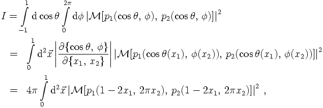
     Consider first a simple two-body decay, filling a two-particle phase space. From the reasoning above, it should be clear that two angles suffice to describe this phase space element, namely cosθ and φ. The Jacobian for this is just a factor of 4π. However, let's try to be a bit more preicese here. To do so, let's assume the decaying particle has rest mass M, i.e., P² = M², and the two decay products have masses m₁ and m₂, respectively. Then, in the restframe of P, the two-body phase space integral can be written as cf. the reasoning above. This allows to rewrite the integration over the two outgoing particles through an integral over the solid angle Ω of particle 1 in the restframe of the decaying particle. Thus, the integration reads and can be replaced by a sampling over random numbers, where with a Jacobian of 4π. From the two random numbers, the three momenta can thus be reconstructed according to, of course, they are back-to-back in the rest frame of the decaying particle. Therefore, the corresponding four-momenta read employing this construction of four-momenta, the phase space integration of a two-particle phase space can be written as a sum,

   • Propagators:

     The next example is a bit more involved, and its importance will become obvious later. However, here's a way trying to explain its significance. Assume that in some reaction an unstable particle is produced and decays further. Due to its limited lifetime, its rest energy (i.e., its mass) are not completely fixed but smeared out. Usually, the mass squared of such an unstable particle, s, is taken to be distributed according to a Breit-Wigner function, where m is the nominal mass of the particle and Γ is its width. This distribution plays the role of a probability density function. Including this into an integral amounts to the formal replacement of the integrator by In other words, instead of integrating over s, the integral is done over F, the integrated p.d.f.. For the sampling this boils down to The task left now is to generate the various sampling points s, over which the summation above runs. In order to select a value of s inside the interval [s_-,s₊] from an uniformly distributed random number R, the following equation has to be solved for s, along the lines of the reasoning above. Simple calculation shows that s is given in terms of R through or by respectively.
     This looks very good: If the integral is over an ill-behaved function g(s), which diverges in the Monte Carlo sense, this behavious may be attenuated by introducing a p.d.f. f(s), which has a similar divergence structure. Due to the ratio in the sampling, the fluctuations then cancel out, leading to a much smoother behaviour of the integrand. However, this has to be taken with a grain of salt: In such a case, the integral over the p.d.f. must be performed analytically and the resulting function must be invertible. Clearly, in most cases which deserve numerical integration, the "true" function g(s) is simpler than the p.d.f. - otherwise there would be no need to integrate numerically.
     The impact of including suitable p.d.f.'s for some simple cases is exemplified here.
   
   
   
4. Smarter sampling methods
   
5. Selection according to a distribution: Unweighting
   
6. Unweighting: Hit-or-miss
   
7. Problems