The Dirac Equation

Schrödinger and Klein-Gordon equation

1. Non-relativistic quantum mechanics: The Schrödinger equation
   
2. Relativistic formulation: The Klein-Gordon equation
   
3. Equations of motion and quantisation
   

   QUANTISING THE HARMONIC OSCILLATOR

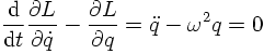
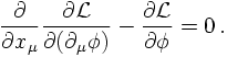
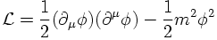
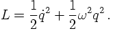
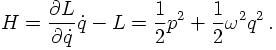
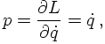
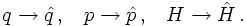
   Recall for a moment how the harmonic oscillator is quantised. Classically, from the Lagrangian the equations of motion (E.o.M.) emerge, namely Also, from the generalised coordinates q, generalised momenta p can be deduced allowing to construct the corresponding Hamiltonian, Quantisation is performed in a series of steps:
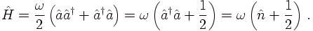
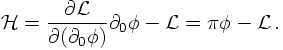
   • The coordinates and momenta, so far merely functions of time, become operators, indicated by a "hat". Of course, also the Hamiltonian becomes an operator:
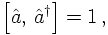
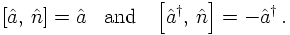
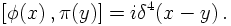
   • Coordinates and momenta satisfy commutation relations (the analogon in classical mechanics are the Poisson brackets): Their E.o.M.'s (time evolution) are given by commutators with the Hamiltonian.
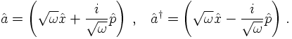
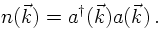
   • Creation and annihilation operators â and â^† are introduced; they can be expressed through the coordinates and momenta by They enjoy the commutation relation with all other commutators between them vanishing, and the Hamiltonian can be expressed through Here, the commutation relations have been used and the number operator has been introduced. Easily, the "vacuum" energy of the oscillator can be recovered. However, the number operator is Hermitean - not a big surprise; after all, the Hamiltonian must be Hermitean as well in order to have real numbers as energies. The interpretation of n as the number operator comes in naturally, just consider its commutators with the annihilation and creation operators:
   
   
   

   E.o.M. FOR FIELDS: RELATIVISTIC GENERALISATION

   The reasoning above, yielding the E.o.M. for the case of a classical harmonic oscillator can be repeated for a chain of oscillators. However, rather than repeating it in detail, which would be part of a lecture on classical or quantum field theory, let us do a reasoning by analogy. First of all, the generalised coordinates, being functions of time, and their derivatives w.r.t. time become the fields, being functions of four-positions, and their derivatives. Since time does not play a special role in a relativistic formulation, the derivatives of the fields are w.r.t. either time or space components, written in Lorentz-invariant form: The Lagrangian becomes a Lagrangian density, written in terms of the fields, which has to be integrated over space-time in order to yield a Lagrangian, Equations of motion can be gained by the analogy of the Euler-Lagrange equations, for relativistic fields they read With this relation, it is obvious that the Lagrangian density for the real scalar field yields the Klein-Gordon equation as E.o.M.. In the following, the term Lagrangian will also frequently be used for the Lagrangian density.
   
   

   QUANTISATION

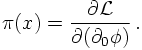
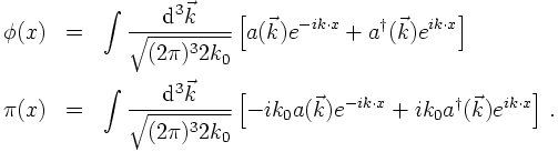
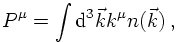
   In order to quantise the Klein-Gordon field, the same reasoning as above applies. First of all, the fields are understood as field operators (hats will be supressed here), and their conjugate momenta are constructed, They can be used to transform the Lagrangian into an Hamiltonian density with the usual trick, Again, coordinates (fields) and momenta (conjugate momenta) enjoy commutation relations; this time however, the commutation realtions are not equal-time but equal-four-position, i.e., The trick now is to go to momentum space, employing a Fourier-transform for fixed times t. transforming the Klein-Gordon equation into an oscillator-like equaiotn whose solution is readily found Here, k₀ is the energy related to the three-momentum k. Since the field φ was assumed to be a real scalar field, its field operator is Hermitean, connecting the two operator q₁ and q₂. Identifiying them with creation and annihilation operators, the field operator and the conjugate momentum become A bit of simple algebra yields the commutation relations for the creation and annihilation operators where all other commutators vanish. Also, a number operator can be defined in a similar fashion as above, for the harmonic oscillator,
   
   

   PARTICLE STATES

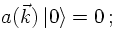
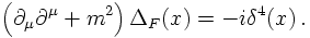
   Equipped with these operators it is simple to construct a basis for the single- and multi-particle states. In fact, the resulting space is called the Fock-space and it is merely a generalisation of the Hilbert-space. Anyways, its vacuum state is defined through the fact that any annihilation operator acting on it yields a zero, particle states are characterised by the three-momenta of the particles populating them (the energies are fixed), and can be produced from the vacuum by repeatedly applying corresponding creation operators, Defining, e.g., a momentum operator through yields, for the momentum of such a state,
   
   

   COMMUTATORS OF FIELD OPERATORS AND PROPAGATORS

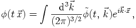
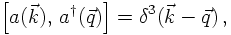
   Using the expansion of the field operators in terms of the creation and annihilation operators, their commutator for arbitrary four-positions can easily be calculated,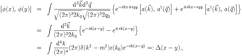 where ε(x) = sign(x) and sign(0)=0. Note thanb in the last line the integration is over all values of k₀, which is only fixed by the on-shell condition. The properties of this commutator Δ are
   • Lorentz-invariance;
   • it is an odd function, Δ(x) = -Δ(-x);
   • microcausality: for x²<0, Δ(x)=0;
   • for equal times it vanishes, i.e. Δ(x) = 0 if x₀=0.
   
   The next thing to be defined and used is the time-ordered product, indicated by a T, It looks a bit funny, but keep in mind that the φ are operators which do not necessarily commute. The vacuum expectation value of this entity is nothing but the Feynman propagator which is used when calculating Feynman diagrams, i.e. transition amplitudes. It can be calculated and yields Here the imaginary part of the denominator, iε, is to be understood in the limit where ε→0; its purpose is to move the poles in the energy integration a little bit away from the real axis. The way this shift is performed reflects the causality structure of the propagator, incorporating an advanced and a retarded piece. This, again, is part of a full lecture on quantum field theory and will not be discussed in any detail here.
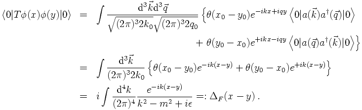
   However, this Feynman propagator is nothing but the Green's function of the Klein-Gordon equation, It can therefore be used to construct general solutions for it.
   
   
4. Equations for a complex scalar field
   
5.