As a first step towards a solution of the instability problem let us analyse the evolution of energy with time:
This explains why the Euler method is bound to fail, irrespective of the size of the time step Δ t. At each iteration, the total energy increases by a positive amount. But, if the method is unstable here, how was it possible to have seemingly stable and sane results in the two previous lectures? The answer is that in general there is not such a thing as "the perfect method" - methods are more or less suitable for different problems. In fact, looking a bit more closely would reveal that the Euler method also led to violations of conserved quantities in those two first examples. But, in contrast to the example here, this was insignificant and could be controlled by choosing the time step small enough. In oscillatory motion, on the other hand, it is often important to discuss many cycles - we will see that later on - and in those cases energy non-conservation, however small per cycle it may be, can accumulate to a larger scale problem. Therefore, since the Euler method fails to conserve energy over the long haul, it must be concluded that in cases like the one at hand it is unsuitable.
So what's the alternative? Of course, the Runge-Kutta method
encountered before does a much better job, and this is the kind of
method that is typically used.
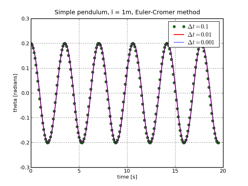
However, instead, let's consider a small deviation of the Euler
method, namely the Euler-Cromer
algorithm, which gives surprisingly good results despite its
simplicity. Compared with the original Euler method,