Let us now make the simple pendulum a bit more realistic by adding dissipation, i.e. a damping force. The assumption typically made in this case is that the friction is proportional to the velocity, such that the equation of motion reads
Since this is still a linear equation, it can easily be solved analytically. The details for the solution can be found in many textbooks on physics; here, it should suffice to state that there are three regimes for the solution, namely
The underdamped regime In this regime the friction is small enough to allow an oscillatory behaviour of the solution, where the amplitude decays exponentially:
where, as before, Ω²=g/l.
The overdamped regime The other extreme is the overdamped regime, where the strength of the friction is so large that the time evolution of the angle is entirely given by an exponential decay,
The critically damped regime At the boundary between these two regimes, the system is said to be critically damped, and the time evolution is given by
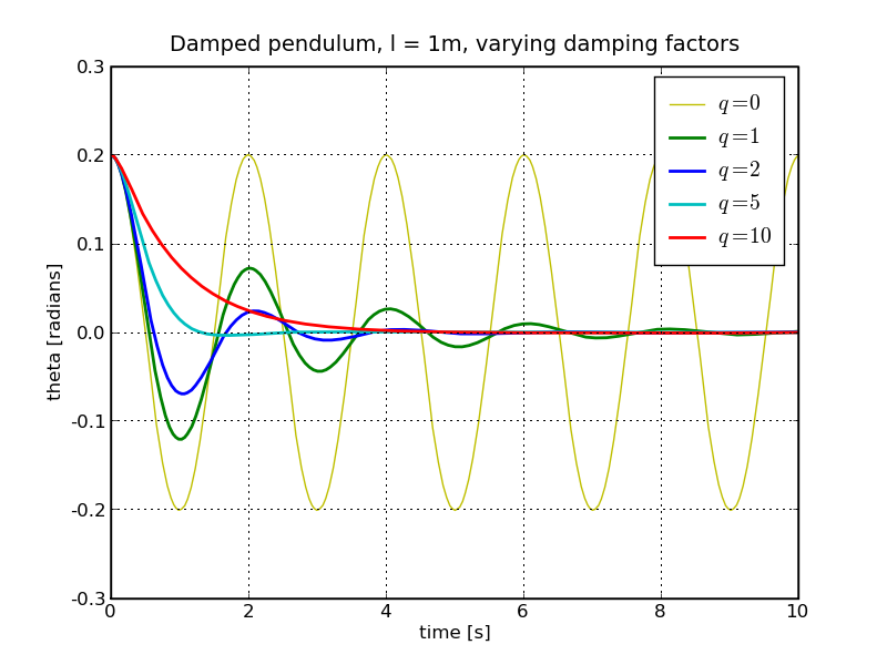
Some numerical results for g = 9.8 m/s², l = 1 m and varying values of q are shown below (for q=5/s the system is close to being critically damped).
Obviously, damping results in the pendulum losing energy, typically as heat.
This is not yet very exciting, so let us add some action. This is best achieved by adding a driving force, which we choose to be of sinusoidal form with fixed amplitude FD and frequency ΩD. Then, the equation of motion is given by
This driving force will pump energy into the system and the driving frequency will compete with the natural or eigen-frequency of the pendulum. It turns out that this equation, too, can be solved analytically, and the steady state solution after "swinging in" reads
where the maximal amplitude is
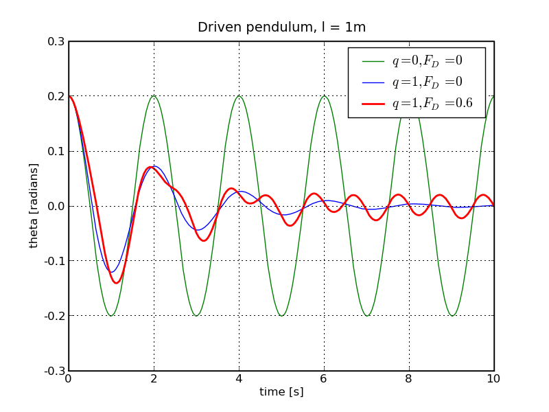
At first sight the driven, damped pendulum shows a somewhat boring behaviour: it just swings with the frequency dictated upon it by the external force. See below for a case where ΩD=2Ω:
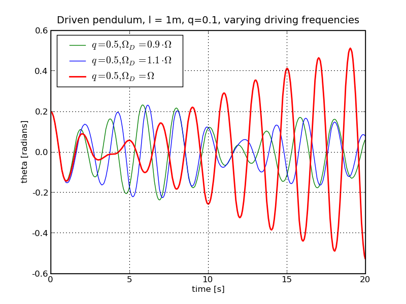
There is an interesting phenomenon, though, namely resonance: the maximal amplitude can become very large in cases where the driving frequency of the external force is identical or nearly identical to the eigen-frequency of the pendulum. This is especially pronounced if the dissipation coefficient, represented by q, is small. Below is the case for FD=0.3 and q=0.1:
The last step towards having a more realistic pendulum is to leave the approximation of small deflection angles. This amounts to not truncating the series
after the first term - which led to our beautifully linear equation of
motion for the mathematical pendulum. Doing that will ultimately
lead to a realistic description of a pendulum and to the emergence of
deterministic chaos.
This subject, however, will be discussed in the next lecture.