Root finding & Integration

Monte Carlo integration and the value of π

We round our discussion of integration methods by introducing a completely different way of doing integrals. This method, known as the Monte Carlo method or Monte Carlo integration builds on using random numbers to do integrals. A prerequisite for this to work is the assumption that we can indeed obtain random numbers (or, actually, pseudo-random numbers) uniformly distributed between some limits. These limits are typically given by [0,1]. In fact, from a computational point of view it is impossible to generate true random numbers, so typically involved algorithms are employed that recursively produce numbers that are, of course, determined by the algorithm in an only seemingly randomised way. Therefore, there's long discussions about the "quality" of such numbers, invoking question of whether the random numbers fill the interval truly uniformly and at which point patterns in the sequence of these numbers start to repeat themselves. Of course, we will not get into the nitty-gritty of such questions and we will happily assume that our random numbers are perfect (which they indeed are for our purposes).

To see how Monte Carlo integration works, let us discuss how the number π can be deduced from integration. One way to look at this is to consider the circle with unit radius. Its area is well-known, A=πr². Knowing the area of this circle in relation to the square enclosing it, allows us to deduce π. So, how can we do this with a random method? Quite simple. Consider a square dart board with dimension 2r, enclosing a full circle with radius r. Throwing darts at this board with a uniform density leads to filling the circle and the space around it with a uniform density. In this case, π can be obtained from comparing the number of arrows hitting the circle with the number of darts that hit the board, including the circle. The ratio of these numbers is equal to the ratio of the respective areas, due to the uniform density.

How can we put this into the computer? Again, this is fairly straightforward. We will restrict ourselves now to the upper right quadrant of the arrangement described above. Orienting it in the x-y plane with the plane's origin on the circle's centre means we consider only the part where both x and y are positive. To keep things simple, we also consider a unit circle, with r=1. Then we can "throw the darts" by letting the random number generator give us two values, one for the x- and one for the y-coordinate. If x²+y²≤ 1 then the "dart hit the circle", otherwise it hit only the board. Counting the number of darts on target and building the ratio with respect to all attempts, N_in/N_tot, will then yield the desired result, the ratio A=π/4.

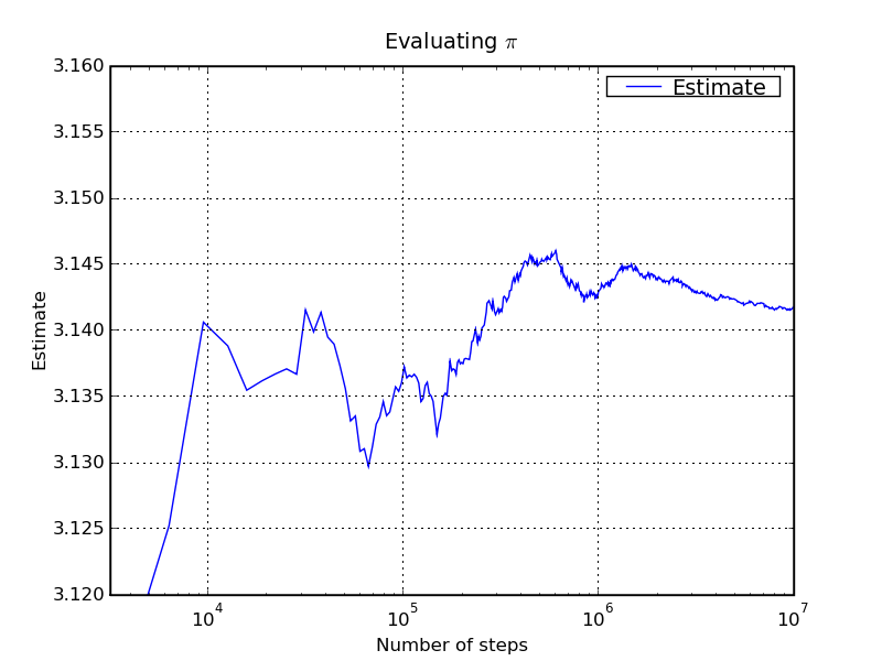
In the plot below we depict how this estimate of π evolves with the number of integration steps, i.e. with the number of points in the Monte Carlo integration.

What we effectively did in this integration was to replace an integral over a function by its average over the interval. For a one-dimensional integral this basic idea can be summarised by

\[I\,=\,\int\limits_a^b {\rm d}xf(x)\,\Longrightarrow \, \langle I \rangle \,=\,\frac{b-a}{N} \sum_{i=1}^N f(x_i)\, , \] In our specific case, we had a two-dimensional integral, with a function \[ f(x,y)\,=\, \left\{ \begin{array}{cc} 1 & \mathrm{if}\,\,x^2+y^2\leq 1 \\ 0 & \mathrm{else.} \end{array} \right. \] Our interval now has a size of 1 (the area spanned by the random numbers, each of which is selected independently in [0,1], replacing the size of the interval b-a in the one-dimensional equation above. So, taken together, we first rewrote the expression for the area of the quarter-circle A as \[ A\,=\,\int\limits_0^1 {\rm d}x \,\int\limits_0^\sqrt{1-x^2} {\rm d}y\,=\, \int\limits_0^1 {\rm d}x \int\limits_0^1 {\rm d}y \, \Theta \left( 1-\sqrt{x^2+y^2} \right) \,=\, \int\limits_0^1 {\rm d}x \int\limits_0^1 {\rm d}y\,f(x,y) \] before we estimated the emerging integral through \[ A\,\Longrightarrow\, \langle A \rangle\,=\, \frac{1}{N} \sum_{i=1}^N f(x_i,\,y_i)\,=\, \langle f \rangle \, , \] where the x_i and y_i are uniformly distributed random numbers in the interval [0,1] each. We introduced here the shorthand of the average of f denoted by ⟨f⟩, without explicitly stating the size of the interval any more.

Having dived a bit into this subject and having started to formalise the subject of Monte Carlo integration in a slightly mathematical language, let us turn to the issue of the error coming with this integration procedure. It is clear that due to the absence of a small parameter - the step-size - there is no way to discuss the size of errors in a language similar to the one used up to now. So let us develop some understanding of the error, and its scaling behaviour. To do so, it is worth noting that, as mentioned above, we try to estimate the integral by repeatedly probing it in a random way and taking the average over the sample made of the probes. This means that we can use concepts of statistics to describe the error. A good way there is to consider the average variance of the sample. It is given by

\[V\,=\,\langle f^2 \rangle-\langle f \rangle ^2 \,\, .\] The square root of the variance is called standard deviation, typically denoted by σ. Assuming a Gaussian distribution of the actual values of f around its mean translates into a probability of around 68% to find the true value of the integral in the interval [⟨f⟩-σ,⟨f⟩+σ] and of around 95% to find it in the interval [⟨f⟩-2σ,⟨f⟩+2σ]. Here, in fact, σ is the normalised standard deviation, 1/N√V. You can find more on this in this wikipedia article. Therefore, we take the normalised standard deviation \[ \sigma \,=\, \langle E \rangle\,=\, \frac{1}{N} \sqrt{V} \] as an estimator ⟨E⟩ on the error in our estimate for the integral.

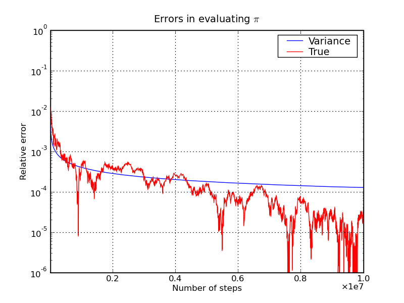
In the plot below, you can see the evolution of this error estimate over integration steps, confronted with the true error, obtained by taking the difference of the estimator of π and its true value.

You can see that the error estimate actually compares quite well with the actual error.

At this point it is worth comparing both approaches to integration, the Newton-Cotes like methods and the Monte Carlo method. Obviously, both types of methods will eventually succeed and produce a result for the integral, and in that respect they're similar. So the interesting question is how the error estimate evolves in time, i.e. with the number of function calls. This clearly depends on the number of dimensions for the panel-type methods, since each dimension necessitates a new factor in the number of panels and hence of function calls. For the trapezoidal rule, using N panels in d dimensions the error scales as N^-2/d, whereas for Simpson's rule the scaling behaviour is given by N^-4/d. Interestingly, due to the statistical approach inherent to it, the error in Monte Carlo integration is independent of the number of dimensions in which to integrate, and it scales like 1/√N. Therefore, for multi-dimensional integration, Monte Carlo methods typically win the efficiency race.

Frank Krauss and Daniel Maitre

Last modified: Tue Oct 3 14:43:58 BST 2017