Scaling is a very useful tool. An equation can be scaled if all variables can be multiplied by the same positive number, which is raised to a different power for each variable, with the equation still holding at the end. This allows the equation to be written as a function of just one variable. In the following we shall discuss scaling and how it relates to the Ising model.
We will begin this discussion with an equation for ⟨s⟩ in the case that \( H \neq 0 \), in a system where each spin has z neighbours with which it interacts.
\[ \langle s \rangle = \tanh\left[ \frac{zJ\langle s \rangle + \mu H}{k_B T} \right] \approx \frac{zJ\langle s \rangle + \mu H}{k_B T} - \frac{1}{3}\left( \frac{zJ\langle s \rangle}{k_B T} \right) ^3 \,\, . \]In this equation, J is the energy of intereaction, μ is the magnetic moment per spin, kB is Boltzmann's constant and T is the temperature of the system. This can be rewritten as a dimensionless equation of state (E.o.S).
In this rearrangement, b and u are positive constants, whereas
\(h=\frac{\mu H}{J}, \, m=\langle s \rangle\) and
\(t=1-\frac{zJ}{k_B T}=\frac{T}{T_C}-1 \) are dimensionless variables. The
value Tc is the critical temperature in mean field theory. This
equation gives the parameter m (⟨s⟩
in the initial equation) in terms of two independant variables.
Taking m as a function of t and h (m(t,h)) we can
create the equation
For all positive values of λ, this equation is true and our dimensionless E.o.S will still hold.
To demonstate the claims above, choose λ=16. This alters our variables: h→8h, t→4t and m→2m. Putting this into the E.o.S yields:
\[ \begin{eqnarray*} \lambda^{3/4} h &=& b\,\lambda^{1/2}t\,\lambda^{1/4}m+u(\lambda^{1/4} m)^3 \\ 8 h &=& b\,4t\,2m + u(2m)^3 = 8(btm+um^3)\,\, . \end{eqnarray*} \]Clearly, the factors of 8 will cancel out to reveal our initial E.o.S. As can be shown in general by the first of the above two equations, this will work for all positive values of λ.
In order to now express our E.o.S as a function of only one variable, we must make a sensible choice for λ. In this case it is |t|-2. Placing this into m(λ1/2t, λ3/4h) yields
\[ m(|t|^{-1}t,\, |t|^{-3/2}h)=|t|^{-1/2}m(t,\, h)\,\, , \]which can be rearranged to obtain an expression for the original function m(t,h),
\[ m(t,h)=|t|^{1/2}m\left( \pm 1,\, \frac{h}{|t|^{3/2}} \right) =|t|^{1/2}f_\pm \left( \frac{h}{|t|^{3/2}} \right) \,\, .\]In this equation the ±'s refer to t > 0 and t < 0, or equally when T > Tc and T < Tc, respectively. This is the scaling form. This equation can be scaled by |t|1/2 to give an expression for m that is solely dependant on one variable, in this case \(\frac{h}{|t|^{3/2}}\).
However, our use of mean field theory has created some problems. We already know that it does not give a good approximation around the critical point, and the predicted critical exponents are not accurate. The general form found above is correct, but a better expression of the scaling form is
\[ m(t,h)=|t|^\beta f_\pm \left( \frac{h}{|t|^{\beta\,\delta}} \right) \,\, . \]This yields the equation found with mean field theory for β = 1/2 and δ = 3
This is an example of an equation that connects power laws with corresponding
critical exponents. Scaling is very useful for such equations and provides a
useful way of describing systems around their critical points.
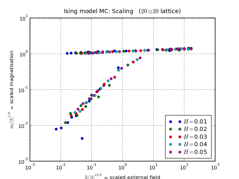
The results obtained from scaling the magnetisation, m(t, h) is
represented below
The upper branch of the diagram represents T < Tc, and the lower branch represents T > Tc
The concept of the renormalisation group is very important to scaling. This describes how systems behave under general scale transformations.