Phase Transitions

In the previous lecture we introduced the Ising model of ferromagnetism. This included a brief overview of a second order phase transition from ferromagnatism to paramagnetism, occurring at the critical point. In this lecture we shall continue the investigation into phase changes, and we shall consider phase changes of the first order in some detail. First order phase transtitions are very common in nature, including the phase change from water to ice, along with other freezing or condensing systems. First order phase transistions are much more abrupt than second order, as there are no prior fluctuations as there are around the critical point. The behaviour of systems around the critical point is often described by a power law with a critical exponent. This critical exponent is thought to be universal, as within experimental error it is equilvent for the Ising model and liquid-gas systems. A technique called scaling is very useful for describing the behaviour of systems around the critical point.

The topics in this lecture are covered in chapter 8 sections 4-6 of Giordano & Nakanishi

Observables

1. Energy
   Continuing with the Ising model, each spin in the system will have a certain energy associated with it. This is dependant on the orientation of the spins with which it interacts. In a very basic Ising model this is just its nearest neighbours. The energy of the total system, therefore, can be caluclated as the sum of the average energy of the constituent spins. This can be calculated using

   \[ \langle E \rangle = -J\sum_{\langle ij \rangle} s_i s_j \,\, , \] where s_i and s_j refer to the spins at locations i and j respectively, and J is the positive exchange constant. As spins pointing in the same direction give a negative energy by the equation above, it can be seen that spins prefer an aligned state. It is also known that:
   \[ \langle E(T=0) \rangle = -NJj/2 \,\, \]

   N = number of spins and the factor of 1/2 occurs because each pair of spins is couted twice, once where 'spin 1' is considered as 'spin i' and once when it is considered as 'spin j'. The term j in this equation is the number of nearest neighbours with which each spin interacts. In the 2D Ising model case, this number is 4. Also,

   \[ \langle E(T\longrightarrow \infty ) \rangle \longrightarrow 0 \,\, ,\]

   as the disorder in spin alignment increases with temperature. Increasing disorder in spin orientation leads to a more random ratio of 'spin up' to 'spin down'. This results in an average energy and magnetic moment of zero.

   The results of a simulation of the Ising model for energy per spin vs temperature is shown below.

   

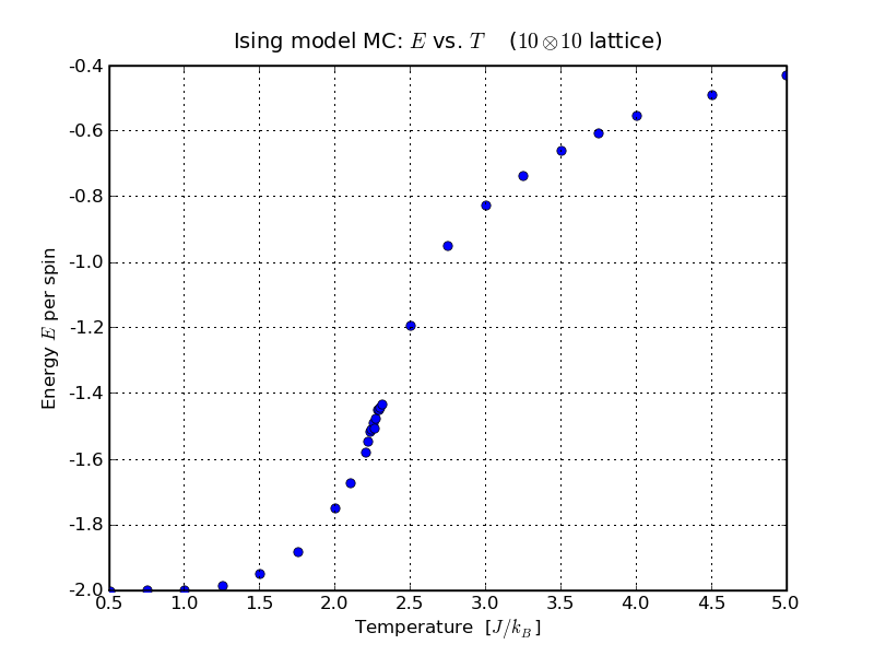
   The negative energy of the spins in this graph occurs because neighbouring spins tend to align. For any given spin in the lattice, it will have a negative energy if it is pointing in the same direction as its neighbours, and positive if it is in the opposite direction. Therefore, a net negative energy for the lattice implies that more spins are aligned in the same direction as their neighbours than opposing. Despite this, the magnitisation of the material at temperatures above T_c is zero. This means the average magnetic moment of the system is zero; there are the same number of spins pointing 'up' as there are pointing 'down'.

2. Specific Heat
   Specific heat is related to energy very closely as its definition is

   \[ C=\frac{\mathrm{d}\langle E \rangle}{\mathrm{d}T}\,\, . \]

   For an infinite system, an energy vs temperature diagram, such as the one shown above, shows an infinite discontinuity in the first derivative of energy w.r.t. time at the point T_c. Therefore, from the definition given above, specific heat has an infinite discontinuity at T_c. The behaviour of the system can be described by the power law

   \[ C \approx \frac{1}{|T-T_c|^\alpha} \,\, \]

   which exhibits the divergence at the temperature T_c due to the inflexion point in the energy. This power law has a critical exponent α.
   The fluctuation-dissipation theorem states that the specific heat can be related to the variance of the energy squared, (⟨E²⟩ - ⟨E⟩²), by

   \[ C=\frac{\langle E ^2 \rangle - \langle E \rangle ^2}{k_B T}\,\, . \]

   The value for ⟨E^m⟩ is obtained from sampling E^m during the sweeps of the lattice. From this equation, the Monte Carlo results for energy vs temperature can be used to estimate the specific heat. This does indeed yield a peak around T_c, and the size of this peak increases with lattice size.
   The results for this analysis of the specific heat for a 10 × 10 lattice is shown

   

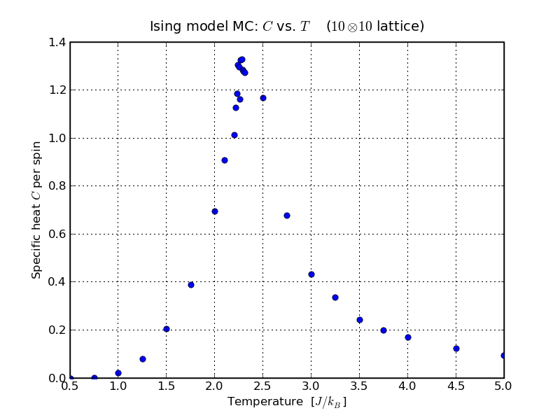
   It can be seen from the above plot that there is a peak at a temperature around T=2.25. This is the temperature that the phase transition was considered to occur in the previous lecture. This is therefore T_c, a point where there would be an infinite discontinuity, and not simply a peak, if the model did not suffer finite size effects.

3. Susceptibility
   This is the measure of the magnetisation, ⟨M⟩, that is introduced by a magnetic field, H. This introduces a new variable, an external field, as previously we have only considered spontaneous magnetisation.

   \[ \chi = \frac{\mathrm{d} \langle M \rangle}{\mathrm{d}H} \]

   Again, the fluctuation-dissipation theorem can be applied, this time introducing a dependancy of the susceptibility on the variance of the magnetisation. This relationship is

   \[ \chi = \frac{\langle M^2 \rangle - \langle M \rangle ^2}{k_B T}\,\, , \]

   The value for ⟨M^m⟩ is obtained from sampling M^m during the sweeps of the lattice.
   χ, in fact, also diverges for the condition T → T_c. This is described by another power law with a critical exponent γ.
   This enables us to investigate how the system would react to an external field without it becoming necessary to actually apply one.

Next→