Newtonian mechanics and equations of motion
← Previous
The origin of algorithmic errors: The Taylor expansion revisited
The Euler method has a number of shortcomings, which are due to its
apparent simplicity. To gain some deeper insight into this, let us
go back to the Taylor expansion of x(t), which was central to
the construction of the method,
\[ x(t\,+\, \Delta t)\,=\, x(t)+
\frac{\mathrm{d}x(t)}{\mathrm{d}t}\Delta t\,
+ \dots \]
According to the
mean value theorem
,
there is a specific value, $t_m$, such that an
exact solution for $x(t+|Delta t)$ can be obtained:
\[ \exists t_m \in [t,t+\Delta t)\, :\,\,\,
x(t+\Delta t)|_\mathrm{exact}\,=\,
x(t)+ \left. \frac{\mathrm{d}x(t)}{\mathrm{d}t} \right|_{t=t_m}\Delta t\,.
\]
In this sense, the choice of $t_m$ incorporates the effect of curvature
(second and higher order terms in the Taylor expansion). Of course,
the best choice for $t_m$ is in general not known, and must thus be
estimated. In the Euler method, the choice is such that $t_m$ is
approximated/estimated by t, the lower edge of the interval
in question. Graphically this translates into interpolating
x(t) by its tangent taken at t.
Better DEq solvers: Runge-Kutta methods
Obviously there are better, more intelligent methods to have a better
estimate of $t_m$. One popular example is provided by the
Runge-Kutta methods. They come in two widely
used variations, as Runge-Kutta method of second and fourth order.
Starting from the first-order differential equation
\[ \dot x\,=\, \frac{\mathrm{d}x(t)}{\mathrm{d}t}\,=\, f(x,t) \]
in the second order Runge-Kutta method x(t+Δ t) is given by
\[ x(t+\Delta t)\,=\, x(t) + f(x',t') \Delta t \, , \]
where the sampling point { x', t' } is constructed as
\[ \begin{eqnarray*} x'&=& x(t)+\frac{\Delta t}{2}f(x(t),t) \\
t'&=& t\,+\,\frac{\Delta t}{2}\,. \end{eqnarray*} \]
In other words, the exact but unknown slope,
$[{\rm d}x(t)/{\rm d}t]_{t=t_m}$, is estimated not by invoking $f(x,t)$
as in the original Euler method, but by the function $f$ taken at some
intermediary sampling point $\{ x', t' \}$, $f(x', t')$. Time-wise,
this sampling point is located in the middle of the $t$-interval, and
its position comes from Euler approximating $x$ to the value
$x(t+\Delta t/2)$.
It can be shown that this approximation indeed is exact up to terms of
the order (Δt)³ in each time step, and therefore
solutions obtained with this method are globally of second order
accuracy. In other words, the total error reduces quadratically with
decreasing Δt.
Of course, there is nothing like a free lunch in this world, and the
price to pay for this apparent improvement is an increased computational
cost, i.e. a longer running time of the program. It is simple to
estimate that this increase consists of roughly a factor of two with
respect to the Euler method since there are in principle two Euler-like
steps per time step. On the other hand, due to its quadratic scaling
of accuracy, the accuracy gain can easily outweigh this cost (since
the Euler method has to run with significantly reduced step size for
the same error).
The approach above can be further improved by estimating the true slope
$[{\rm d}x(t)/{\rm d}t]_{t=t_m}$ through a weighted average of several
terms of the form $f(x'_i, t'_i)$ with $i = 1,2, ... $, with the times
$t'_i$ suitably chosen in the interval $[t,t+\Delta t]$ and with the
positions $x'_i$ obtained from some Euler-approximation from $x(t)$.
A popular (and in fact the most wide-spread DEq solver) choice is the
fourth-order Runge-Kutta method defined by
\[ x(t \,+\, \Delta t)\,=\,x(t)+\frac{1}{6}
\left[ f(x_1',t_1')+ 2f(x_2',t_2')+2f(x_3',t_3')+ f(x_4',t_4')\right]
\Delta t\, , \]
where the sampling points $\{ x'_i, t'_i \}$ are constructed as
\[ \begin{eqnarray*}\begin{array}{lcllcl}
\displaystyle
\vphantom{\frac{|^|}{|^|}}
x'_1 &=& x(t)&
t'_1 &=& t \\
\vphantom{\frac{|^|}{|^|}}
x'_2 &=& x(t)\,+\,f(x'_1,t'_1)\frac{\Delta t}{2}&
t'_2 &=& t\,+\,\frac{\Delta t}{2} \\
\vphantom{\frac{|^|}{|^|}}
x'_3 &=& x(t)\,+\,f(x'_2,t'_2)\frac{\Delta t}{2}&
t'_3 &=& t\,+\,\frac{\Delta t}{2} \\
\vphantom{\frac{|^|}{|^|}}
x'_4 &=& x(t)\,+\,f(x'_3,t'_3)\Delta t&
t'_4 &=& t\,+\,\Delta t \, .
\end{array}\end{eqnarray*} \]
It can be shown that the local error of this approximation indeed is of
order (Δt)5, leading to a global error of order
(Δt)4. This increased accuracy motivates to live
with a computational cost of roughly four times the original Euler method
per step. However, due to the increased accuracy, this is a burden which
is usually acceptable, rendering the 4th order Runge-Kutta method the
approximation of choice.
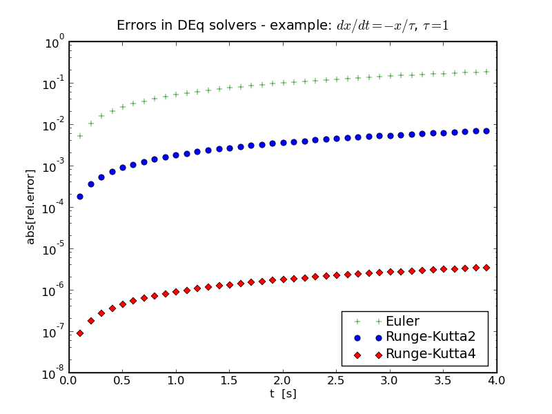
Euler vs. Runge-Kutta
After your homework, all three methods for solving a differential
equation of order one have been implemented. Below, they have been
used to the differential equation describing radioactive decay,
\[ \frac{\mathrm{d}x}{\mathrm{d}t}\,=\,-\frac{x}{\tau} \, , \]
where τ=1 has been chosen. The relative errors of the various
methods w.r.t. the known analytical result are exhibited below and
exemplify drastically the advantage of using the Runge-Kutta methods.
 Daniel Maitre has produced a wonderful set of
slides
with some excellent animations and further insights.
Daniel Maitre has produced a wonderful set of
slides
with some excellent animations and further insights.
Next →
Frank Krauss and Daniel Maitre
Last modified: Tue Oct 3 14:43:58 BST 2017