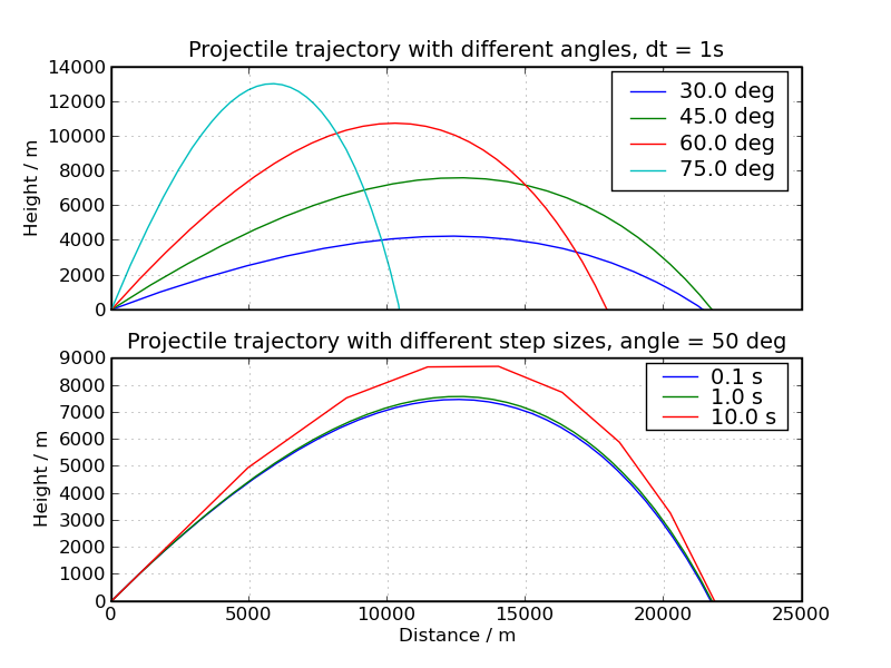
Newtonian mechanics and equations of motion

Euler method for the solution

The starting point for the implementation of this problem and its solution in the form of a computer code is the following set of equations

\[ \begin{eqnarray*}\begin{array}{lclcl} \displaystyle \dot{x}\,&=&\,\frac{\mathrm{d}x}{\mathrm{d}t}&=& v_x \\ \dot{y}\,&=&\,\frac{\mathrm{d}y}{\mathrm{d}y}&=& v_y \\ \dot{v_x}\,&=&\,\frac{\mathrm{d}v_x}{\mathrm{d}t}&=& -\frac{B_\mathrm{drag}vv_x}{m}\\ \dot{v_y}\,&=&\,\frac{\mathrm{d}v_y}{\mathrm{d}t}&=& -g-\frac{B_\mathrm{drag}vv_y}{m} \end{array}\end{eqnarray*} \] After discretisation we have a series of time steps (and corresponding positions and velocities) \[\begin{eqnarray*} t_i\,&=&\, t_0\,+i\Delta t=i\Delta t,\,\,\,\,\, i\in{\{0,1,2,\dots\}} \\ x_i\,&=&\,x(t_i),\,\,\,\, y_i\,=\,y(t_i),\,\,\,\, v_{x,i}\,=\,v_x(t_i),\,\,\,\, v_{y,i}(t_i) \end{eqnarray*} \] Then, the equations of motion above can be approximated as \[ \begin{eqnarray*} x_{i+1}\, &=&\,x_i + v_{x,i}\Delta t \\ y_{i+1}\, &=&\, y_i + v_{y,i}\Delta t \\ v_{x,i+1}\,&=&\,v_{x,i}-\frac{B_\mathrm{drag}v_iv_{x,i}}{m}\Delta t\\ v_{y,i+1}\,&=&\,v_{y,i}-g\Delta t - \frac{B_\mathrm{drag}v_iv_{y,i}}{m} \Delta t \, , \end{eqnarray*} \] where, of course, \[ v_i\,=\, \sqrt{v_{x,i}^2 + v_{y,i}^2} \, . \] The only thing left to be done then is to fix the initial conditions, which in this discretised form read \[ x_0\,=\,y_0\,=\,0\,\, , \,\,\,\, v_{x,0}\,=\,v_0\, \cos\theta\,\, , \,\,\,\, v_{y,0}=v_0\, \sin\theta \, , \] such that the firing angle and the muzzle velocity become the input parameters.
Adding in the calculation of the range of the shot, the pseudo-code for this problem thus reads

Main program
In the main program, the steering unit, the following tasks will have to be fulfilled:

Input the parameters of the program.
Initialise the class "Cannonball", encapsulating the physics problem and the class "DEq_Solver" for the actual calculation.
Use the latter to solve the differential equation and produce results.
Store and plot the results.
Initialise the class "Interpolator" and estimate the range of the shot with it.

Initialisation of the physics problem
(encapsulated in the class "Cannonball")
The following parameters etc. need to be read in:

$v_0$, the muzzle velocity,
$\theta$, the firing angle,
$B/m$, the drag coefficient of the projectile,
$\delta t$, the timestep size, which again is a parameter of the calculartion and not of the physics.

We assume that g is fixed by $g = 9.81 {\rm m/s}^2$.
Also, fix the initial conditions:

$t_0=0$,
$x_0=y_0=0$,
$v_x = v_0\cos\theta$ and $v_y = v_0\sin\theta$.

Calculation: Solution of a general differential equation of first order
(encapsulated in the class "DEq_Solver")
The calculation amounts to the following algorithm:

Repeat the time steps outlined below with size Δt until $y_{i+1}\le 0$.
In each time step:
1. calculate $t_{i+1} = t_i+\Delta t$;
2. calculate the components of the acceleration due to the air drag force:
  $\underline a_{\rm drag} = \frac{\underline F_{\rm drag}}{m} = -\frac{B_{\rm drag}}{m} v_i\underline v_i$,
  using the velocity components of the step before.
3. employ the equations above to update positions and velocities:
  \[\begin{eqnarray*} x_{i+1} &=& x_i+v_{x,i}\Delta t\\ y_{i+1} &=& y_i+v_{y,i}\Delta t\\ v_{x,i+1} &=& v_{x,i}+a_{drag,x}\Delta t\\ v_{y,i+1} &=& v_{y,i}-g\Delta t+a_{drag,x} \end{eqnarray*} \]
4. calculate the absolute value of the (updated) velocity $v_{i+1}$;
5. store the time, positiions, and velocities.

It should be noted that, in principle, this is already provided in your class DEq_Solver, the only thing neccessary is to realise that the components of the positions and velocities form a vector $\underline x = (x,y,v_x,v_y)$ (stick to exactly this sequence!) and to provide a corresponding function $\underline f$ in the class "Cannonball".

Range estimate
A simple linear interpolation for the range of shot should be sufficient.
To this end, we interpolate between $y_{i+1}$, the first point where $y<0$, and $y_i$, the last point were $y>0$ yielding

\[ x_\mathrm{range}\,\approx\, \frac{x_i+rx_{i+1}}{1+r}\, , \,\,\,\,\, r=-y_i/y_{i+1} \, . \] Of course, here $y_{\rm range}=0$.

Results with the Euler method

Some results obtained with this example code are shown below. A more interactive version necessitates the following two additions: code for inputs of angle, velocity etc. and the steering code. Obviously, the naive expectation of maximal range at an angle of 45 degrees is altered by the effect of the air resistance - you can check this by not looking at the plot but rather running the code yourself. To highlight the effect of air resistance it also makes sense to increase the drag factor from 0.00004 to a higher value. Note also how the precision of the results changes with the step size dt.

Frank Krauss and Daniel Maitre

Last modified: Tue Oct 3 14:43:58 BST 2017