Harmonic motion
Harmonic motion is a frequent phenomenon in physics, and not surprisingly
the study of harmonic motion in its different aspects constitutes one
of the first encounters with theoretical physics, and it continues to be
a subject at higher levels. Perhaps the simplest mechanical system
that exhibits harmonic motion is the pendulum, consisting of a mass
connected through a string with some hook to support it. As soon
as the mass is brought out of its equilibrium position it is allowed to
freely swing back and forth under the influence of gravity. In the
highly idealised case of small deflections, i.e. small angles, from
equilibrium and frictionless motion this system indeed exhibits
harmonic motion. The main features of this motion can found in
many other systems, mechanical, electromagnetic, and so on, and this
renders the simple mathematical pendulum the paragon example of this
kind of motion. Typically then, some other features are added to the
discussion, namely a driving force and some damping.
However, most undergraduate textbooks stop at this stage.
In this and the next lecture we will set out for a numerical treatment
of real oscillatory systems. Starting with the highly idealised case
of a frictionless mathematical pendulum we will discuss how to
treat simple harmonic motion. Having sharpened our tools, we will then
include the effect of friction and a driving force. In the next lecture
we will add non-linearities to the system and observe how it is
driven into chaos. While chaos has some intuitive meaning for all of
us (typically inherited from mums describing our rooms), it is hard
to define it in a quantitative, physical manner. By struggling with
this definition we will recover some key issues for the description of
chaotic systems.
The subject of this lecture is also discussed in chapter 3,
sections 1 and 2 of Giordano & Nakanishi.
The simple physical problem and its analytical solution
|
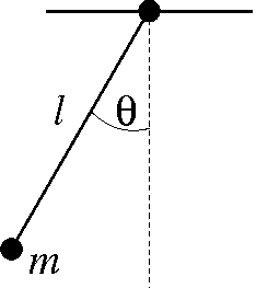
Assume a pendulum with mass m, connected with a fixed
support through a rigid massless rod of length l.
The deflection angle θ is taken with respect to a
vertical line, such that the equilibrium position of the mass is at
θ=0. The conjugate angular velocity will be denoted by
ω. Gravity is directed vertically, but due to the rod
its effect amounts to a force perpendicular to the rod, driving the
mass into its equilibrium position,
\[ F_\theta\,=\, -mg\sin\theta\, \approx\, -mg\theta \,\, . \]
Here, the approximation in the force is valid for small angles - it
is the first term in the Taylor expansion of sinθ.
Newton's law then implies the following equation of motion for the
mass in terms of the deflection angle:
\[\ddot{\theta}\,=\, \frac{\mathrm{d}^2\theta}{\mathrm{d}t^2}\,=\,
-\frac{g}{l}\theta \,\, . \]
|
|
There's a variety of equivalent ways to write the solution of this
equation, the one chosen here reads
\[ \theta (t)\,=\, \theta_0\sin(\Omega t+\phi)\,\, , \]
where Ω=(g/ l)1/2 is the angular eigen-frequency
- up to a factor of 2π identical to the eigen-frequency -
of the pendulum, and &theta0 and φ are
constants representing the initial deflection and velocity of the
pendulum.
The emerging pattern of motion is in fact very simple:
sinusoidal oscillations in time, continuing forever with constant
amplitude. This is no surprise, since ignoring the effect of friction
translates into a constant energy of the system. In the same limit
of small angles used before, the total energy is given by
\[ E=E_{\rm kin}+E_{\rm pot}=
\frac{m}{2}l^2\omega^2(t)+mgl[1-\cos\theta(t)]\,
\approx\,\frac{m}{2}l^2\omega^2(t)+\frac{m}{2}gl\theta^2(t)\,\,. \]
From this equation we see how energy is shuffled back and forth between
kinetic and potential energy. Using the fact that ω is
given by dθ/dt the energy thus is
\[ E\,=\,\frac{mgl}{2}\theta_0^2 \,\, , \]
clearly a constant.
Next →
Frank Krauss and Daniel Maitre
Last modified: Tue Oct 3 14:43:58 BST 2017