PHYS4181 Particle Physics - Phenomenology
These are the notes for the third instalment of the 4th year course Particle Physics PHYS4181. In a series of 12 lectures we will become familiar with the known spectrum of elementary particles, their interactions and properties and how do we study them in the laboratory. This course reaches till the edge of known physics and it stands on previous necessary knowledge. The audience is presumed to have been introduced to relativistic quantum mechanics and gauge theories. What one is expected to come out of here with is knowledge of our present theory of elementary particles, the principles it is based on, the symmetries and conservation laws it presents, and how to connect it with experimental observations. In less lofty and more practical terms we will learn about conserved charges, Feynman rules and phase space integrals.
These lectures are meant to be self-contained to a large extent but a useful short bibliography is:
-
[2]
Quarks & Leptons, M. Halzen & A. Martin
-
[5]
Modern Particle Physics, M. Thomson
-
[1]
Introduction to Elementary Particle Physics, D. Griffiths
-
[6]
Elementary Particle Physics in a Nutshell, C. G. Tully
in addition to previous years materials available on DUO.
Self-assessed problems will be made periodically available and so will their solutions a week later, you have ten days to work on them and send your self-assessment. The schedule is at www.dur.ac.uk/resources/physics/students/level4weeklyproblems.pdf. Some of these problems can be found on these notes as footnotes but they will be collected in the problem sheets as well. In addition workshops will be held on Fridays to solve a different set of problems and your queries about the self-assessed problems.
Both for the purposes of easing you into the subject and starting soundly anchored in reality, we open with an historic review and look at the experiments that took us where we are today.
Outline of lectures
The approximate schedule for the lectures is,
-
•
Lecture 1 Brief historical introduction to particle physics and overview of the course material.
-
•
Lecture 2 Collider characterization and kinematics. The CMS experiment as an example of a particle physics detector.
-
•
Lecture 3 Theory perspective, path integral and fundamental action. Review of Feynman rules.
-
•
Lecture 4 The Standard Model: particle content, fundamental Lagrangian and conservation laws.
-
•
Lecture 5 Quarks as constituents of the proton, deep inelastic scattering.
-
•
Lecture 6 Hadronic and partonic cross section connection, parton distribution functions.
-
•
Lecture 7 Quantum Chromodynamics, . Asymptotic freedom.
-
•
Lecture 8 The Electroweak interactions, . Chirality. Mass vs interaction eigenstates: bosons.
-
•
Lecture 9 Electroweak gauge boson properties from collider experimental data.
-
•
Lecture 10 Spontaneous symmetry breaking. Higgs boson properties from collider physics.
-
•
Lecture 11 Mass vs electroweak interaction eigenstates, fermions. Flavour Physics of quarks and leptons.
-
•
Lecture 12 Beyond the Standard Model.
1 A brief history of particle physics
The history of particle physics is, as that of physics in general, not a straightforward affair but full of twists and turns, dead ends and awe inspiring leaps in knowledge. While this makes for an entertaining read, see for example the first chapter in LABEL:Bk:G, it can also be misleading to the uninitiated looking to understand the established physics that came out of the historical process. So here we will be rather selective in our choice of discoveries and theoretical ideas to highlight so as to fit best our current simple picture which describes nature, the Standard Model (SM). The purpose here is to acquire some culture and familiarity with the particle spectrum and the observations that built it.
We start back in the late 1940s, the scientific community has discovered that atoms are made of electrons orbiting around nuclei themselves made of protons and neutrons and the photon is the building block of the electromagnetic field, but further, the positron, discovered in cosmic rays by Carl D. Andersen, has been identified as the antiparticle of the electron predicted in Dirac’s equation. In 1947, where we start our timeline in fig. 3, C. F. Powell and his co-workers at Bristol cleared up the confusion around the new particles seen in the impact of cosmic rays (basically protons) with the atmosphere. Making use of photographic emulsion they identified two kinds of particles, muons () and pions (). 11 1 Pions are more frequently seen the higher up and some of these emulsions were placed in the top of mountains. Can you make sense of why muons make it further down the atmosphere than pions by looking at their basic properties? You can assume they both are produced at the same rate and with equal velocity. PDG site, pion PDG site, muon. While the pion had been predicted as the mediator of nuclear interactions by Hideki Yukawa, the muon was unexpected, (I.I. Rabi is quoted as saying ‘Who ordered that?’, if he only knew what was coming!). Cosmic rays were to bring surprises in the form of new particles that same year, G. Rochester and C. Butler published a cloud chamber photograph displaying a particle decaying into pions; the Kaon had been found. The 50s saw a frenzy of new particle discoveries in what quickly grew to be a long catalogue, … see http://pdg.lbl.gov/ for our current list. Some of these particles behaved like heavier pions and were termed mesons while other seemed heavier versions of protons or neutrons and were called baryons.
To make sense of it, M. Gell-Mann and G. Zweig theorised the existence of quarks, three of them: up, down and strange, which both mesons and baryons (collectively denominated hadrons) were made of. This interpretation put some order in the particle zoo arranging them in multiplets of a symmetry group. It is interesting to remark from this historical viewpoint that, like most of the theory milestones of fig. 3, in the inception of the ideas that make up the Standard Model they were often not taken seriously, at times by the authors themselves, and it took many years to develop them into their present form. So despite the fact that deep inelastic scattering experimental data from Stanford Linear Accelerator (SLAC) by the late 60s provided evidence for the proton being composed of smaller objects, it would take another particle discovery for the theory to take shape. The components of the proton were termed partons in R. P. Feynman’s interpretation of deep inelastic scattering, which were later identified with quarks and gluons. On the theory side the quark model was taken one step further by M. Gell-Mann and H. Fritzsch with the formulation of what we now call quantum chromodynamics (QCD), a gauge theory, while in 1973 D. Gross, D. Politzer and F. Wilczek discovered the asymptotic freedom of the model.
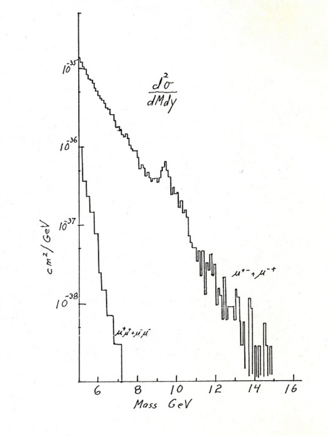
In November of 1974 the discovery of the particle was announced simultaneously by collaborations of experiments at SLAC, lead by B. Richter, and Brookhaven National Laboratory (BNL), lead by S. Ting. A hectic period in particle physics ensued out of which the quark theory would emerge as the model for hadrons. The new particle could be accounted for with the addition of a fourth quark, charm, already proposed in the work of S. Glashow, G. Iliopoulos and L. Maiani in 1970. The addition of this quark implied not only the presence of the but other particles which were indeed found experimentally. A few years later in 1977 evidence for a fifth quark presented itself in the discovery of the Upsilon by L. Lederman et al. at the experiment E288 in Fermilab. Further evidence in support of the quark model and QCD came in 1979 from three jet events at the TASSO experiment at PETRA collider, in Deutsches Elektronen Synchrotron (DESY). These events arise from the emission of a gluon, the mediator of the gauge interaction in QCD. The last quark to join the ranks is the heaviest, the top quark, discovered at the TeVatron in Fermilab in 1995.
The physics of leptons and the weak interactions developed in the same era but it is conceptually useful to separate it from the history of strong interactions. The muon was in the particle catalogue by 1950 but the electron neutrino was only detected in 1956 via inverse nuclear beta decay by C. L. Cowan and F. Reines at the Savanah River nuclear reactor. The neutrino had been theorised by Pauli in the 30s to carry the missing energy in beta decay but in another example of the growth of theories it had to wait 20 years to be recognized as a real entity. As we know today the muon has its own partner muon neutrino but in the late 1950s the presence of a single neutrino in nature was a possibility. L. Lederman, M. Schwartz, J. Steinberger and collaborators at BNL found a source of muon neutrinos from pion decay interacted with protons to produce muons but no electrons. It was concluded that the partner neutrino of the muon was different from the electron neutrino of beta decays and added to our elementary particles. History and nature would repeat themselves when the tau lepton (), a heavier version of the muon just like the muon is a heavier version of the electron, was discovered in the mid 70s at experiments lead by M. L. Perl at SLAC and Lawrence Berkeley National Laboratory (LBL) whereas the tau neutrino was detected by the DONUT collaboration at Fermilab in the year 2000.
Beta decay as well as the decay of taus and muons into lighter particles was known to be mediated by a ‘contact’ interaction distinct from the electromagnetic or strong forces; it was described by E. Fermi’s theory of the 30s. This theory was known to be incomplete at higher energies which lead Glashow and Weinberg and Salam to seminal works during the 60s. These works accounted for the contact interaction by introducing a vector boson mediator, the boson, which originates from a gauge theory. These models predicted not only the particle producing charged currents interactions and decays but also another massive gauge boson, the , which induced ‘neutral current’ interactions. These neutral current interactions were measured by the Gargamelle bubble chamber at CERN in 1973. The electroweak theory, although supported by experiments, did not have direct confirmation in the form of detection of the predicted and bosons. It was CERN again with the efforts lead by C. Rubbia and S. Van der Meer in the experiments UA1,UA2 on the Super Proton Synchrotron (SPS) that announced within months the discoveries of the and the bosons in 1983.
The weak interaction was therefore based on the same gauge principle as the strong and electromagnetic interactions yet with the crucial difference that electro-weak bosons were massive. This required a mechanism for the mass generation of elementary particles in addition to the gauge principle or the theory would be inconsistent at higher energies. A simple mechanism for mass generation was proposed in 1964 by P. Higgs, R. Brout and F. Englert and G. Guralnik, C. R. Hagen and T. Kibble which took the name of the former. The prediction of this mechanism was a scalar particle which coupled to the rest of elementary particles proportionally to their masses. Corroboration of this idea clocks in as the longest with almost fifty years between the seminal works and the discovery of the Higgs boson at CERN in 2012.
2 The LHC as a particle physics experiment
The experimental techniques and methods in particle physics have evolved throughout the years and often had spin-off developments that helped shape society as we know it today (e.g. the www was developed at CERN). Again we cannot do justice to it all but simply give here a very simple sketch of a modern particle accelerator.
Both in photographic emulsions and cloud chambers used as particles detectors in the 40s and 50s charged particles could be seen by the tracks of ionized material they left when traversing the detector. These detectors in the infancy of particle physics used cosmic rays as a source but with the advent of particle accelerators one could control the production as well as detection. Linear and circular, fixed target and center of mass accelerators have been built and together with ever-more-advanced detectors produced the results that fueled particle physics. The basic physics of detection and production however are not hard to grasp and here we jump to a current experiment to serve as pedagogical example.
Colliders are characterized in simple terms by two quantities: center of mass energy and luminosity L; let us start discussing . Consider two free particles in collision course with momenta
| (2.1) |
where we have chosen our unit of speed as the speed of light, i.e. and . What is the energy available in the collision to, for example, produce new particles? Part of the total energy, , is translational and due to the system moving as a whole, so a different observer moving at a relative speed sees momenta:
| (2.2) |
where is the transpose velocity (a row vector) and the projectors are explicitly P and P. To determine the energy available for the ‘reaction’ one can do as in classical mechanics and sit on the center of mass frame. In order to do this we find the Lorentz transformation, that is , such that the total 3-momentum vanishes in the new frame , then the total energy in this frame is the internal energy available. This exercise leads to the CM energy which can be expressed in terms of the original 4-momenta as22 2 Derive this equation by finding the boost that takes to the center of mass frame, that is solving and later substituting in .
| (2.3) |
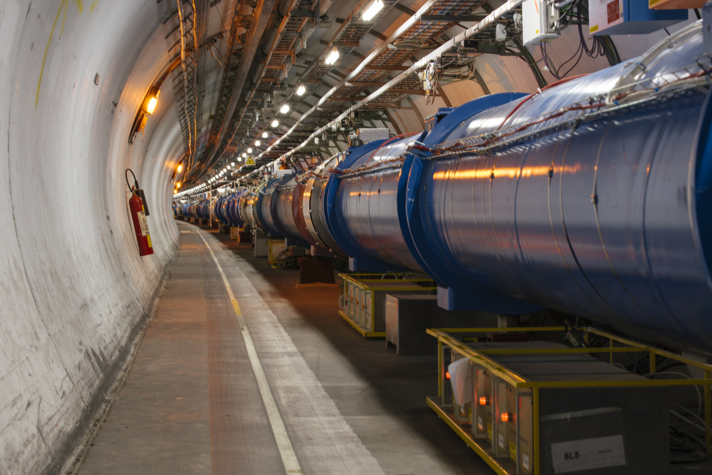
So no matter what rest frame we find ourselves in, we can find the center of mass energy by the Lorentz contraction of (, which is a Lorentz invariant33 3 In a fixed target experiment a beam collides into a static target, for example take static protons and TeV energy electrons; the center of mass energy is then .. Indeed whether a collision of a positron and an electron can produce a muon and anti-muon is something which all observers can agree on. The collider that will serve as example here is the Large Hadron Collider (LHC) at CERN. The LHC accelerates two streams of protons travelling in opposite directions (and so the laboratory frame is the center of mass frame) in its 27 kilometre ring to an energy of TeVeV each for a CM energy of TeV. When the two beams of protons meet some of them will interact and possibly produce observable signals in the detectors. Let’s look at one of the protons in one of the beams with momentum , the probability that this proton interacts with the other beam when he traverses it during a time interval is
| (2.4) |
where F is the flux of particles from beam 2 per unit time ([F]=), that is the number density of particles times the relative velocity. The other factor, , is the cross section and can be thought of as the area around a particle within which particles going through will interact (but note that the cross section depends on what particle we are scattering with). Then beam 1 has itself protons so the probability of some interaction or event to occur is
| (2.5) |
where L is called the instantaneous luminosity, proportional to the flux and the number of particles of each beam. This parameter we can control experimentally, as opposed to the cross section, which is given by fundamental physics.
The beams at LHC are however not a continuous but they are separated into bunches, some circulating in each direction. Per bunch crossing then in formula (2.4) we obtain the probability of a proton to interact substituting the time that it takes him to traverse the other bunch , taking the bunch to be a cylinder of length and volume , so . There are protons per bunch, the same on each beam (), and approximately whereas given that they travel at nearly the speed of light and the LHC ring is 27km long, they go through the interaction point with a frequency of km s. Altogether this yields a luminosity of , given that the beams are squeezed via quadrupole magnets to an area of m one can estimate the LHC luminosity at around nbs were a barn (b) is a unit of area equal to cm.
Luminosity is therefore measured in (length) (time) and the cumulative luminosity over time is called integrated luminosity, L. The LHC has collected in what is called run 2 (2015-2018) an integrated luminosity of around inverse femto-barn (fb). This represents a huge amount of data, some trillion collisions yet if we are interested in a particular process, like Higgs production, we have a much smaller data set. Let’s do an estimate of Higgs production, given the Higgs production cross section ,
| (2.6) |
These events are recorded in the detectors placed at the collision point. At LHC there is not just one collision point but four, where the detectors ATLAS, CMS, LHCb and ALICE are placed.
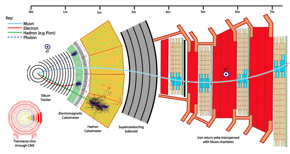
ALICE studies heavy ion collisions and LHCb b-quark physics. The two multi-purpose detectors are CMS and ATLAS and we describe here CMS as an example. It is 211515m in size and 14,000 tons heavy with most of its weight coming from a superconducting solenoid (circling 18.500A!) that produces one of the strongest magnetic fields ever manufactured. We can see a transverse view of the detector in fig. 5. There are four main components in the detector each with different functionality.
-
1.
The inner part of the detector is the tracker where particles trajectories can be identified and traced back to the vertex where they originated from. Since it has a powerful background magnetic field, charged particles curve and their momenta and charge can be measured.
-
2.
In the next encapsulating shell we find the electromagnetic calorimeter (ECAL) which stops electrons and photons and measures their energy.
-
3.
Surrounding the electromagnetic calorimeter the hadron calorimeter (HCAL) is where hadrons (pions, kaons, protons etc) are stopped and their energy measured. A given process produces a lot of hadrons in the direction of the original parton, this is called a jet and they are the way in which we ‘see’ partons after collision. At the same time it is designed to be as hermetic around the interaction region as possible so as to identify missing energy events.
-
4.
Lastly muons make it through all the previous detectors and are identified in the muon chamber which contains a strong magnetic field and where muon momenta momenta and charge is measured.
With all the information collected from the detector we try to reconstruct as much as possible the kinematics of the elementary interaction that mediated the scattering.
3 Path integral and Feynman rules
In this lecture we turn to the theory formulation in particle physics. The formalism chosen here is based on the path integral; first we introduce this concept in quantum mechanics to next apply it to Quantum Field Theory (QFT) and finally summarise our results in the form of Feynman rules and formulae for observables.
The events in our collider of choice depend on cross sections which are given by phase-space integrals of squared scattering amplitudes, themselves derived from a fundamental action. The action is the spacetime integral of the Lagrangian density ,
| (3.1) |
where denotes collectively the fields associated with particles one is studying, e.g. a neutrino field . In particle theory models for nature are often discussed in terms of their Lagrangian which, since the rise of QFT, has played a central role. The connection between Lagrangian and cross sections and decay rates is not a simple one nonetheless; here, rather than focus on rigour, we sketch the basics of the formulation (and the way to sidestep it). To guide our intuition through the math, let us anticipate that the action controls the evolution of a system and hence the range of possible outcomes in our experiment.
Here are some of the questions that (perhaps) have occurred to you and we will try to address. You are familiar with the Lagrangian from classical mechanics and the derivation of equations of motion but how does it show up in quantum mechanics? And why would we rather talk about Lagrangians over Hamiltonians as one does in quantum mechanics? To answer these we use a path integral, which you might not have seen before, so let us present it in its simplest realization.
Path integral in quantum mechanics
Take a canonically quantized system with operators , and eigenstates , , as you are familiar with from quantum mechanics:
| (3.2) | ||||||
| (3.3) |
You can think of and as position and momentum in one dimension, but they could be other conjugate variables of our system, and we will eventually take them to be field and conjugate variable . Take an initial state at some time , and let us compute the possibility that it ends up in a different state after a time . The time evolution is given by the Hamiltonian
| (3.4) |
where we assumed a time independent Hamiltonian and it can be thought of as kinetic plus potential energy for a non-relativistic object moving in one dimension with unit mass. The amplitude we are considering then has a simple expression:
| (3.5) |
Next we break the time in intervals and insert a number of ‘identities’ to evaluate the operators in terms of eigenvalues.
| (3.6) | ||||
Lets break it down to each of the pieces
| (3.7) | ||||
| (3.8) | ||||
| (3.9) |
The argument of the exponential is
| (3.10) | ||||
| (3.11) |
We can carry out the integral in since it is a Gaussian which we know gives in general
| (3.12) |
so that
| (3.13) |
and the amplitude reads
with and where we can identify the finitesimal derivative of in and the Lagrangian in half its square minus the potential . This finitesimal version of the Lagrangian is multiplied by the increment of time so taking the infinitesimal limit we can write:
| (3.14) |
with
| (3.15) |
The path integral takes a little getting used to. A given ‘point’ in the space we are integrating over is given by the value of at the different times. One can plot this as in fig. 6; with time on the horizontal axis and on the vertical axis, we specify the ‘point’ by the values of in the vertical axis at each time. If we join these values with a line, which must start and end at respectively, we have ourselves a ‘coarse-grained’ function or a ‘path’ from to which in the limit does turn into a function. Well, there you go, the path integral is an integral over functions, or in our physical interpretation paths from the initial to the final state, where we note that these functions do not even have to be continuous or differentiable. The contribution of different paths to the final outcome is dictated by the action which acts as a weighting factor.
This integral is not possible to evaluate in general, but certain limits are somewhat intuitive and of physical importance. Consider a neighbourhood around a given function with a non-vanishing variation of the action ; contributions around this point can both increase and decrease the action and hence have phase factors that tend to cancel out. By contrast around a configuration with the fist contribution is given by the second variation, which for a minimum, gives a same-sign coherent contribution. But this configuration we know, its the solution to Lagrange’s equations! This means that the classical path is a potential good point around which one can expand the path integral. Whether it is a good expansion in practice depends on our system but one can formally take the limit to suppress all other contributions and recover classical mechanics from the path integral.
In general nevertheless we sum over all paths and it is the action that determines the final result, the evolution of the system. From here already one can see the importance of the action and Lagrangian. Finding the fundamental action (or equivalently Lagrangian) that describes the world at its most elemental is the key to predict and understand the possible phenomena and outcomes in nature. This makes the case for the theorists fixation with Lagrangians; there is the hope that the search for new phenomena and particles will yield a complete description of Nature which will be specified by ‘The Action’. At present we know that our current theory given by the Standard Model action is incomplete. But lets come back down to the specific physics we are concerned with here, smashing particles together, which is one of our ways to search.
Path Integral in Quantum Field Theory
The connection with particle physics and quantum field theory is obtainable by translation, take a scalar field for example
| (3.16) |
where the difference is now we have fields and hence another label on top of time: space and so is a Hamiltonian density. This leads to an action
| (3.17) |
The main difference and where we require a bit more work is that the states are not the final states we are looking at. Canonical quantization prescribes that the operator creates and annihilates particles, in particular
| (3.18) |
where is a particle state with momentum and hence the eigenstate of , , is a superposition of multiparticle states. It will also be convenient, given our focus on scattering of momentum eigenstates, to Fourier-transform our fields to momentum-space.
Given orthogonality of momentum states (which we assume), eq. (3.18) tells us that the insertion of creates a particle, made explicit in the decomposition of the field in terms of creation and annihilation operators which nonetheless we do not need here. One has therefore that insertions of the operator in between the vacuum state must be related to the transition probabilities involving particles (some of coming in some of them going out).
This requires that in our path integral we also allow for powers of the field ‘downstairs’ while the final and initial states are taken to be the vacuum. Instead of computing the possible path integrals separately here we borrow a method from statistical mechanics and define the partition function starting from
| (3.19) |
which would be the th order integral. The source is introduced as an extra term in the action
| (3.20) |
so that taking derivatives with respect to we bring down ’s which we interpret as creating and annihilating particles and antiparticles.
If one knows how to perform the integral, the theory is solved, that is we can make exact predictions. However in general one does not know how to solve this integral and perturbation theory is our way to make progress. This is based on some basic integrals which we do know how to perform, case study a Gaussian integral.
Let us illustrate this with the scalar action of eq. 3.17 and the two-point correlator,
| (3.21) |
where functional derivatives are defined by . Let us rearrange the action as
| (3.22) |
where we used integration by parts, , we define to satisfy and a shift in the dummy integration variable has been used. This result back in the path integral
| (3.23) |
where we have identified the path integral in as . We managed to compute a path integral (!) and obtained as the answer so let us have a closer look; it is a function of two spacetime points and defined to be an inverse as:
which is the propagator for a scalar field; all we had to do to ‘compute’ the path integral is to invert the operator of the quadratic action (in ).44 4 If you are acquainted with the cannonical formalism in QFT you have seen a propagator before, yet here it acquires a new interpretation in terms of expectation values of fields, relevant in early-time Cosmology.
In our interpretation however this result should be connected to a transition probability between momentum eigenstates, first a Fourier transform yields
| (3.24) | ||||
| (3.25) |
We can interpret this result if we flip one of the momenta which is equivalent to taking the particle outgoing; then this expression is only non-zero if the initial and final momenta are the same which is what we can expect of a transition amplitude. There are however extra factors which require an overall normalization for this to be interpreted as a matrix element. This normalization involves the propagator itself as a more rigorous consideration yields.
The derivation of this normalization can be found in books on QFT, e.g. section 7.2 of [4], here we borrow the result so we can finally connect momentum-space path integrals with scattering processes. Let us denote the amplitude for a transition from incoming particles to a final state with particles as the matrix element of the scattering matrix , , and , our derivation leads us to: 55 5 This expression is valid to first order in our perturbative expansion, the next order (one-loop) introduces a field renormalization factor, both here and in eq. (3.18), which we omit.
| (3.26) | ||||
| (3.27) | ||||
| (3.28) |
The first line above is known as the Lehmann Symanzik Zimmermann reduction formula [3] and there is a lot to unpack here. What we mean by disconnected is best understood with a diagrammatic approach as in fig. 7, disconnected are processes in which some particles travel freely and do not talk to the rest of particles which corresponds to letting act on the free piece exp. As for the derivation we have used the same trick as for the propagator, introducing and using and in the last step we specify that the derivation is to be taken with respect to the Fourier transformed field and and opposite-sign-momentum transformed for incoming and outgoing particles respectively .
To get acquainted with this expression let us take the following interaction
| (3.29) |
and look into 2 to 2 particle scattering with incoming momenta and outgoing momenta . This means now taking the derivative that the out-states have flipped momenta:
the path integral on cancels out with the factor in the denominator and we have therefore obtained the (first order in ) matrix element. It is conventional to define the invariant matrix element as
| (3.30) |
with the sum over initial and final momentum respectively. We found then ; that was a lot of work for a simple result, lets look at a different process next and see if the final answer is equally simple. Next say the case of proton with field scattering off an electron via the electromagnetic interaction ()
| (3.31) |
so the matrix element is computed from
| (3.32) | ||||
| (3.33) | ||||
we can perform the path integral in perturbatively which is precisely the propagator
| (3.34) | ||||
| (3.35) | ||||
| (3.36) |
which again has an overall momentum conservation Dirac delta and ends up being simpler than the derivation machinery might have suggested. To connect the above with the matrix one still has to contract with spinors which are the connection between field and particle state. The ones we will need in these notes go only up to spin 1. They are
| (3.37) | ||||||
| (3.38) | ||||||
| (3.39) | ||||||
| (3.40) | ||||||
| (3.41) | ||||||
| (3.42) |
where is a complex spin one ( vector-boson) field and , .
This gives us for our electron-proton scattering .
Feynman rules
Nevertheless the simplicity is indicative of a shortcut to the result which is simply a collection of rules which one can gather after doing a number of computations like the above. The directions for this shortcut are known as Feynman rules
-
1.
Interaction vertices To derive the Feynman rule for a given vertex take the derivative of the interaction term in the Lagrangian with respect to fields until you obtain a constant and put an into it. Complex fields are treated as independent fields. The vertex is represented diagrammatically by each of the fields being a line joining in a point. We have seen a couple of examples
.
-
2.
For a initial/final state particle () with momentum and spin one must supplement the derivative w.r.t. to the field with the field-state connection, this means a factor ()
-
3.
For internal lines which connect two vertices we put in the propagator , these are:
-
4.
For a given process draw all possible diagrams (to a given order in your perturbative expansion) matching the external states. For each diagram write with the rules 1-3 while imposing momentum conservation on each vertex to fix the momenta of propagators as much as possible. Make sure is a Lorentz invariant by ensuring all Dirac and Lorentz indexes are added up, in particular for Dirac indexes one can use matrix notation (where order matters) by starting from the end of a fermion line and continuing up against the arrow. The final result is the sum of for each diagram.
It can be shown that all diagrams at first order (called tree level) in our perturbative expansion have the momenta of propagators fixed in terms of the momenta of external state. The next order does not and there’s internal momenta which we have to integrate over (we call this loop momenta and loop integrals).
These are the rules, but one only really learns how to use them with examples which is what we will do on the workshop.
Finally, we can take the invariant matrix element and give the cross section, for two particles colliding with four-momenta , and producing particles in the final state:
| (3.43) |
where we recall . The terms inside the integral except for constitute the Lorentz invariant phase space sometimes just called LIPS, whereas the factors out front are related to our normalization of states . On the other hand a decay rate in the particle’s rest frame is
| (3.44) |
with the four momenta of the decaying particle, .
So at last our trip from action to observables is done.
Completion relations
A number of useful relations for the square of the matrix elements when we sum over spins are:
| (3.45) | ||||||
and since , , we have e.g.
| (3.46) |
Finally some relations for gamma matrices which will be useful are
| (3.47) | ||||||
| (3.48) |
4 Standard Model overview
Our last lecture took us all the way from Lagrangian to cross sections, so now that we know the path let us present the starting point (Lagrangian) to the best of our knowledge. This is the Lagrangian of the Standard Model, our description of nature at its most elemental.
Gauge group
At the center of the Standard Model formulation sits the gauge principle. Here we assume the reader has some familiarity with the principle and do not review it. We start by specifying the SM group and the consequences that follow from its formulation. The group is divided into colour, weak isospin and hypercharge, the latter two ‘contain’ electromagnetism in a way which we will make explicit later on. Invariance of space-time dependent (gauge) transformations requires the introduction of gauge bosons: spin-1 massless particles, one for each generator. This means
where II is the identity and are the couplings of color, weak isospin and hypercharge respectively, the only three parameters of the gauge group. The matrices and can be taken as the Gell-Mann and Pauli matrices respectively with the normalization and . The field strengths for the gauge bosons transform in the adjoint representation and are defined as:
| (4.1) | ||||
| (4.2) | ||||
| (4.3) |
The way in which gauge bosons couple to matter is through the covariant derivative, for example if it acts on a fundamental representation of color, weak isospin and hypercharge we have
| (4.4) |
this would be the case for example of left handed quarks but more in general when the covariant derivative acts on a field which is not charged under color the field would be absent, if instead it is not charged under weak isospin would be absent, etc. Therefore to know how the gauge bosons interact with the rest of particles, matter, we have to specify their charges (representations).
Matter
By matter here we understand fields charged under the SM gauge group, which means fermions and the Higgs doublet. As we will see this distinction becomes a bit blurry after electroweak symmetry breaking, but let’s not get ahead of ourselves.
To talk about fermions we have to revise first chirality. As you might know:
| (4.5) |
with the left and right-handed projectors. They are projectors because , , , . The usefulness of this projection is that it commutes with Lorentz transformations, that is, because
| (4.6) |
and commute with the Lorentz group generators. This means that after a Lorentz transformation a left-handed field stays a left-handed field and so does a right handed. That is why we define
| (4.7) |
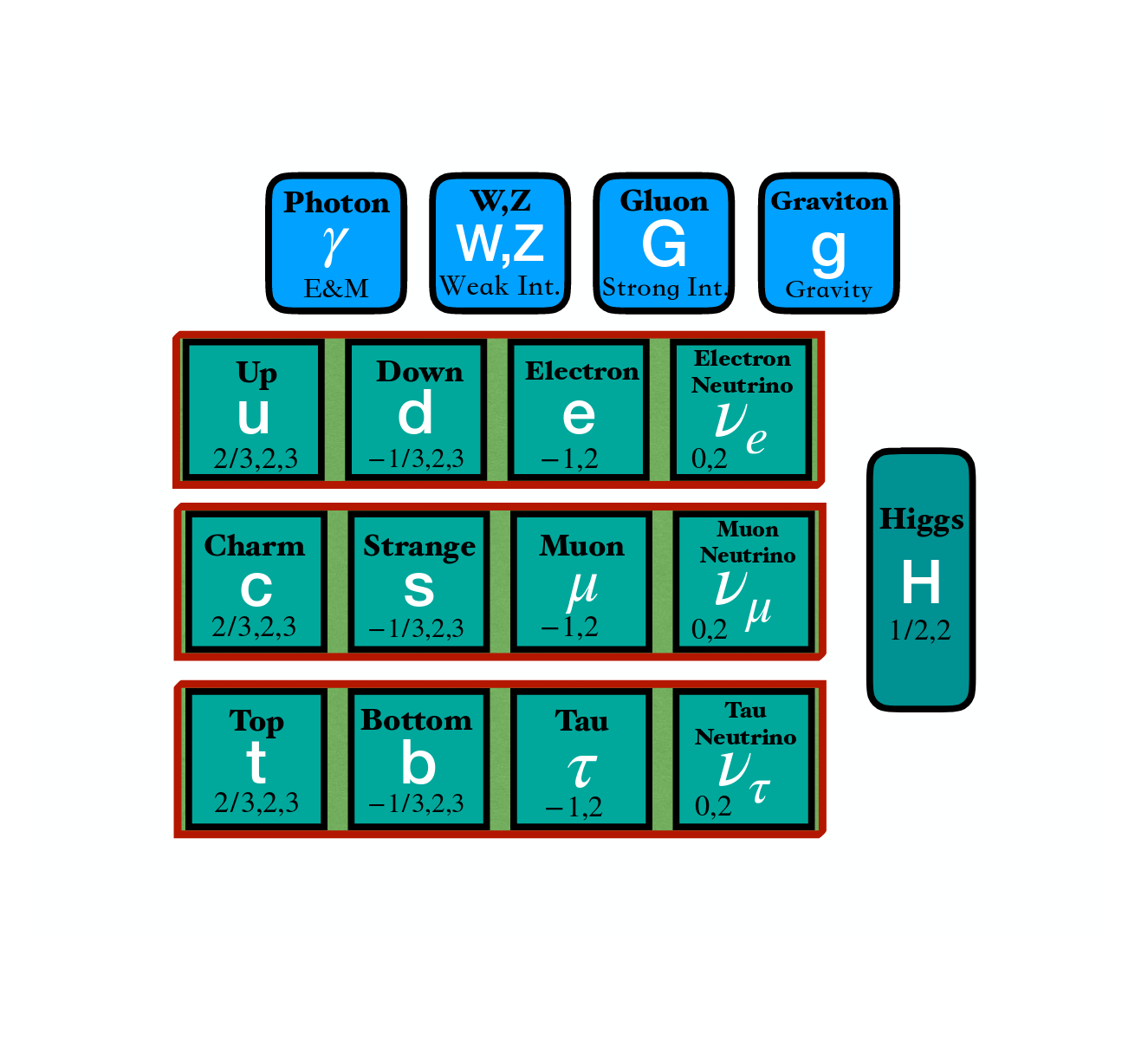
which are irreducible representations of the Lorentz group, the ‘smallest’ fermion. You are familiar with the electron which is made of a left-handed and a right-handed component, but again to get there we must go through mass. For now we split our fermion fields between LH and RH. In the Standard Model there is a total of 5 of them for the first generation, , , , and . Their charges are
where means not charged and a means a fundamental of or , that is a complex vector in 3 or 2 dimensions. This is a significant distinction with the abelian and non-abelian cases, for the former the charge is a real number but for the latter charge is a ‘representation’ and they are a discreet set. One can be explicit about the representations and write the ‘vectors’ out:
| (4.8) |
where r,b,g stand for the three colors (red, blue, green) whereas for each component of the two vector merits its own name, - and - and the subscript gives the hypercharge. Above we have also included the Higgs doublet which as such has 2 complex components (4 real) inside it. So all in all the matter content is given in table 8.
With this much information one can already write a large fraction of the action.
Lagrangian
As we’ve emphasized all throughout, the spacetime integral of the Lagrangian dictates the evolution of our system and possible outcomes and is the central construction from which we derive observables. One might think that if it controls and ‘knows’ about all possible outcomes of say a collision, the Lagrangian of our theory of nature must be a complicated object with many variables and many moving parts. With our present knowledge we can say that is not the case, the Lagrangian of the Standard Model is remarkably simple.
The two rules we follow when building our action are Lorentz and gauge invariance. These symmetries imply conserved currents which we have tested to impressive accuracy; e.g. electric charge is conserved in every process we know of; any non-gauge-invariant term in our Lagrangian would contradict this fact.
The particle content we know of is in table 8, so we can start writing its free Lagrangian, , … but this is not gauge invariant, we have to promote to as in eq. 4.4 which simultaneously tells us how matter and gauge bosons interact. Then we write the part of the Lagrangian which we call including matter and gauge boson kinetic terms :
| (4.9) |
where the sum on fermions is over and and the extra in the in field strengths is related to the normalization for traces and . So for example from the above we can deduce that the quark interaction with a gluon reads .
There is one key aspect that the gauge Lagrangian does not account for: some particles are massive, including part of the gauge bosons. This seems in stark contradiction with the gauge principle so we have ourselves a conflict. The conflict is resolved by the Higgs doublet and spontaneous symmetry breaking. In a nutshell this means that even though our full theory possesses a symmetry, the vacuum state alone does not. We will expand on this in a few lectures time but for now we want to write the part of the action that will do this job. First a simple potential for the Higgs will give it a value in the vacuum different from 0, :
| (4.10) |
and next the Lagrangian terms from which the mass of fermions originates, the Yukawa interactions:
| (4.11) | ||||
| (4.12) |
where
| (4.13) |
which transforms as a 2 as well but with opposite hyper-charge66 6 Check that transforms as a doublet, i.e. given the infinitesimal transformation in substitute in to find .. After electro-weak symmetry breaking, the Yukawa terms will produce masses for fermions as .
Let’s collect all the terms then in the SM Lagrangian
| (4.14) |
This is it. Our Lagrangian for a single generation has 3 gauge couplings, 2 parameters in the potential and three Yukawa couplings. This we fix after looking at experiment and we have input for all of them at present.
| 1.2 | 0.65 | 0.36 | 246GeV | 0.13 | 1.4 | 2.9 | 3.0 |
The one aspect we omitted here is the generational structure of matter. That is a simple extension however, one can put an index in the fermions that runs from one to three so e.g. .
This introduces more parameters in the Yukawa couplings which now are matrices. This we will look into in lecture 11.
Global symmetries and charges
This action was built to respect the gauge symmetries and so via the Noether theorem electric charge is conserved in any process. In addition this theory has other symmetries which are somewhat unintended. You might check yourself that if we give a phase to all quarks (LH and RH and all generations) the Lagrangian in eq. 4.14 stays unchanged. This symmetry we call global because it is only conserved if we make it space-time independent, as opposed to gauge symmetries. Nevertheless it implies a conserved charge, baryon number which we define as
| (4.15) |
The above is meant to include all generations of quarks, so all quarks have Baryon number . Anti-quarks have opposite charge and the rest of elementary particles are neutral under baryon number. This charge is coming from an Abelian symmetry which makes it easy to find the charge of composite objects as
| (4.16) | ||||
| (4.17) |
So mesons have baryon number and baryons have baryon number . This charge is conserved in all process which we have observed in nature, and we have been actively looking for its failure. It also offers an easy check on whether a given process is allowed in the Standard Model, for example, is allowed by baryon number?
About leptons we have a similar result, but stronger even. We can rotate the each different generation with a different phase so we have three different charges: electron lepton number, , muon lepton number and tau lepton number , defined as
| (4.18) |
whereas antiparticles have the opposite-sign charge. These charges, together with electric charge (the other unbroken Abelian charge) offer a simple rule to check whether a given process can happen in the standard model. Here are some for you to train:
| (4.19) | ||||||
| (4.20) |
A key question before moving on is why do we stop in just the terms of eq. 4.14 when writing our action. In our natural units the fields have dimensions of mass to some power (Mass), this power is, respectively
| (4.21) |
you can amuse yourself to find that all terms in the Lagrangian have, when adding up the dimensions of the fields and derivatives, dim. This fact which might seem a coincidence out of the way in which we built our action is actually a very important factor. Field theories which satisfy this condition are ‘closed’ under quantum corrections and very predictive (in our jargon they are called renormalizable).
Finally this action cannot be complete because we have evidence of new phenomena, e.g. neutrino have a mass (which imply that individual Lepton number is not conserved), there is another type of matter out there (dark matter), the universe is in an accelerated expansion phase (dark energy) and we have not included quantum gravity in our picture.
5 Deep inelastic scattering and partons
Quarks and gluons (partons) are not observed as final states in our experiments yet we said they are the components of mesons and baryons and hence nuclei. What is the evidence we have of this being the case? Quite some, here let us discuss deep inelastic scattering as one example which also has historical relevance.
Consider shooting electrons at protons at very high center of mass energy, in particular higher than the proton mass GeV. At this energies the electron can probe the internal structure of the proton and ‘catch’ an unsuspecting parton which behaves like a free particle. This parton receives a large momentum transfer and breaks away so that the outcome, after hadronization, is that the proton has ‘broken’ into various other hadrons.
To see how experimental data can tell us whether this picture is correct, let us start computing the scattering at the partonic level, for concreteness let’s pick an u quark and the scattering . Let’s assume the quark carries a fraction of the total momenta of the proton, then the partonic process is
| (5.1) |
with and we use to denote partonic quantities. Recall the formula for the cross section, which in this case we can simplify a bit since we have relativistic particles ( we take )
| (5.2) |
If one works on the phase space for the final parton
| (5.3) |
where . The lepton phase space one can rewrite changing variables from , in the C.M. to , as
| (5.4) |
where we also integrated over the angle () knowing that the amplitude does not depend on it. For the matrix element, since we do not know the spin of the the particles involved, we average over incoming and sum over outgoing as:
| (5.5) |
we put it together and find
| (5.6) |
Now comes the part that we cannot compute; what is the probability of the photon bumping into a parton with fraction of momentum ? This is a magnitude for whose estimation perturbation theory does not work, yet that does not deter us, we just give it a name: parton distribution function and sum over it,
| (5.7) | ||||
where we used the Dirac delta to set , and found appropriate to change variable from to . Finally we know it’s not only the u quark in the proton but also the so we add it up too
| (5.8) |
where by in the final state we mean summing over all products of the collision, being inclusive. Although we do not know a priori this is still a predictive result which we can test against data.
The general cross section without assuming anything about the components of the proton, only using eletromagnetic gauge invariance reads
| (5.9) |
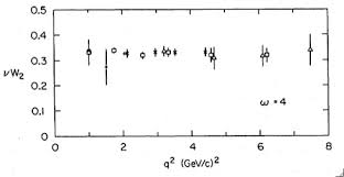
With arbitrary functions of . Stare at eqs. 5.8 and 5.9 for a minute. Even if we start from arbitrary parton distribution function we cannot obtain arbitrary , for one only depends on . Expressed in terms of the conditions that follow from our quark description read
| (5.10) |
with the charge of the parton in units of e ( for , ). This relation is known as Callan-Gross equation. The fact that the functions depend only on is known as Bjorken scaling and a way to test it is to extract from experiment and plot them for fixed and varying , if they do not change the Callan-Gross relation holds and the quark model prediction is right. You can check how well this holds in fig. 10.
6 PDFs and Hadronic vs Partonic
Our study of deep inelastic scattering showed that we can write the cross section for the process, with meant to be anything that can be produced, as an integral over the partonic process times a function of the fraction of momenta
| (6.1) |
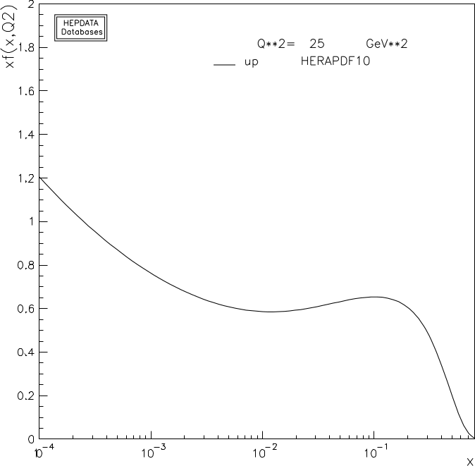
These functions are called parton distribution functions and their extraction from experiment (we cannot compute them) provides a window into the proton inner structure. Let us refine our picture of the proton by contrasting with the pdf of the quark displayed on fig. 11 which we took from our own hepdata website at Durham.
|
|
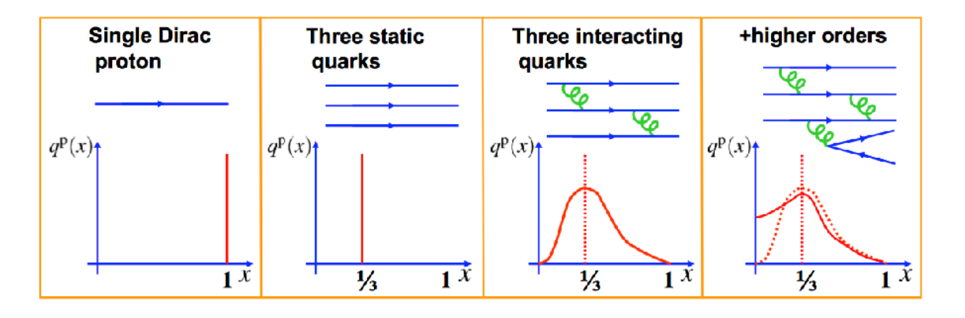
We see that the function peaks around but the most salient feature is that at low , does not vanish. This means that the total probability diverges since at , what have we missed? We only considered the proton as 3 quarks sitting still and not the interactions that keep them together, the plot in figure 11 is a stark reminder of how simplistic this view is. As we now know QCD is the theory that describes the interactions and, although it this regime we cannot compute using it, it still provides a description to make sense of the results.
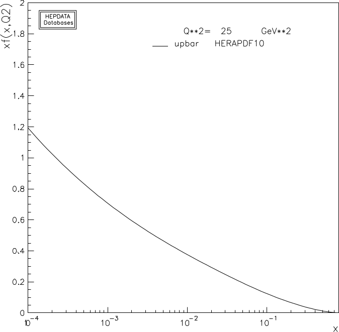
In our starting picture each quark would carry one third of the momenta and so its pdf would look like a peaked function around . Nevertheless quarks ‘talk’ to each other exchanging gluons and hence momenta back and forth which means that they do not have a precisely defined value of momenta and the width of the peaks broaden. In addition virtual processes occur like the emission of a gluon and his splitting into a quark anti-quark pair. It could then be that our photon encounters this quark. This we typically consider ‘unlikely’ since in perturbation theory this emission requires more powers of the coupling and is sub-leading. However, in this regime ! the logic of perturbation theory does not apply and this is the mechanism that produces the rise in for , we encounter up quarks popping out. These are called sea quarks as opposed to valence quarks. A consequence of this picture nonetheless is that if the low ’s come out of a quark-anti-quark splitting, there should be antiquarks around too. There are, and they have their pdf which we plot in fig 11. Our intuition for the component quarks then applies to the difference, since the sea quarks and anti-quarks must have the same pdf
| (6.2) | ||||||
| (6.3) |
Another integral result is that the total momenta must be the sum over all parton pdfs times the fraction of momenta they carry, if we include strange quarks which are also present, this means
| (6.4) |
Well, we can do the integral on the RHS and, for example, at we find the result is 1/2. There is something missing which the scattering of electrons off protons does not see. A neutral parton…
That is right, the gluon, the gluon is the missing parton in our counting. One indeed has the gluon pdf and as we shall see it is the gluons that are responsible for most of the production of Higgs bosons at LHC.
As you might remember, at LHC we collide protons and protons. How do we obtain the hadronic or ‘real life’ cross section from the partonic process in this case? Well there will be two pdfs involved now and a double sum over partons. So the total cross section reads.
| (6.5) |
where denote the different partons. We have made explicit the dependence of the partonic cross section on the external CM energy . Why do we evaluate the partonic cross section at ? Let’s work out the kinematics, the partonic CM energy is
| (6.6) | ||||
| (6.7) |
since at the LHC energies we can neglect to a very good approximation the mass of partons GeV vs (10TeV). The center of mass energy then at the elementary process is a fraction of the total energy. Given that at these energies the pdfs peak to low , it also explains why even if the LHC is nominally set at 13TeV very little of the events carry the full energy.
7 Quantum chromodynamics
Thus far we have seen evidence for the proton made of quarks but also neutral partons carrying a large share of momenta which we called gluons, as well as anti-quarks. This gives us an inventory of elementary particles that make up hadrons, yet, how do they interact is something we have not quite discerned yet.
Red blue and green
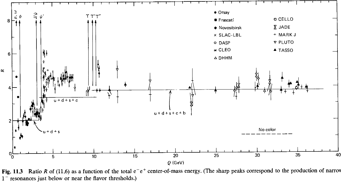
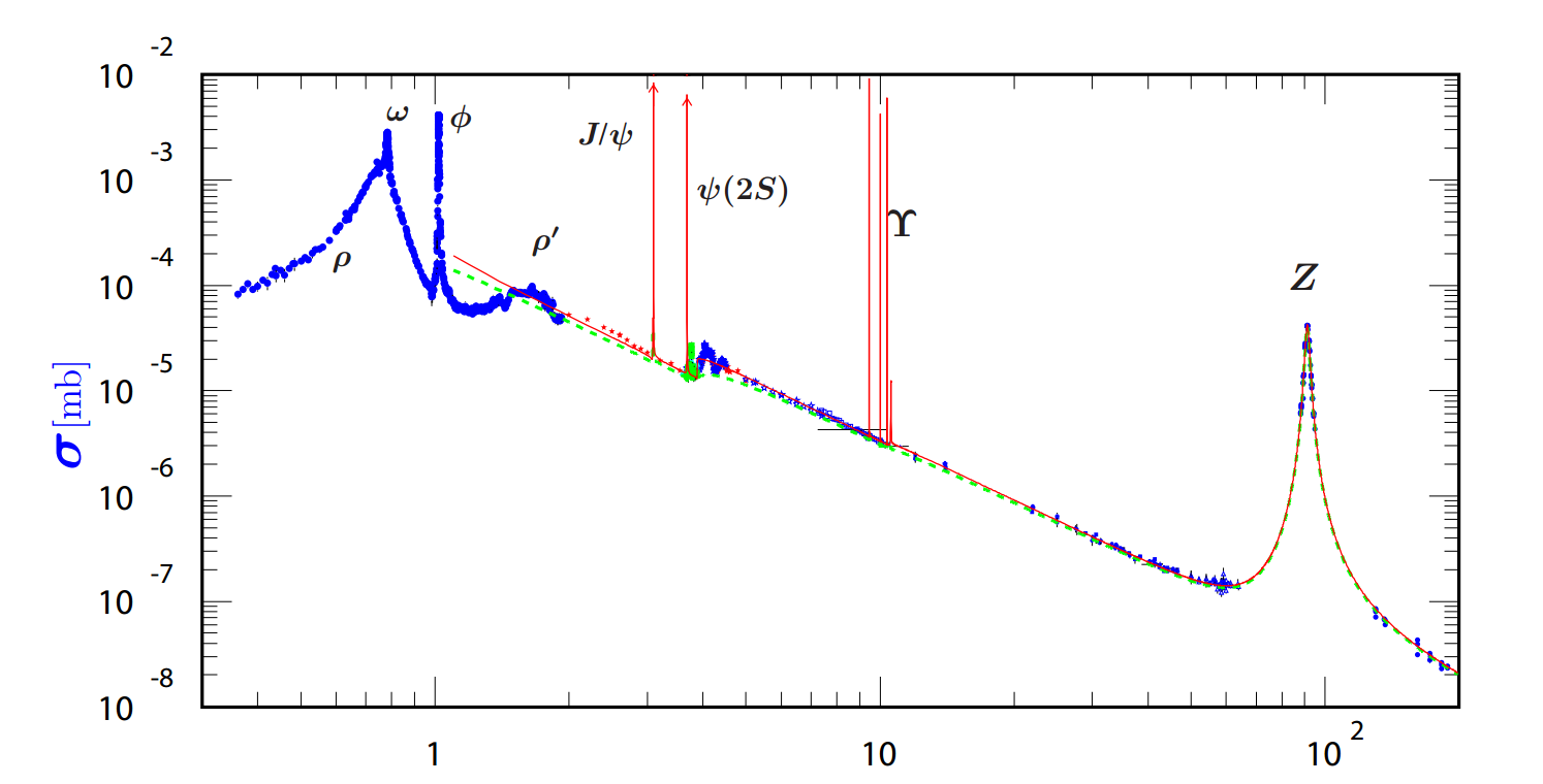
For starters how do we know it is ? Consider an experiment like that at PETRA accelerator at DESY where positrons and electrons where made to collide. They can annihilate and, at low energies through a virtual photon, create pairs of whatever particles have electromagnetic charge and are available for production (i.e. ). This has the matrix element
| (7.1) |
Take the annihilation into a muon, this has a cross section, sitting in the C.M. frame and approximating all particles to be massless as
| (7.2) |
where we have used the fact that in the CM and , we have averaged over initial-state spins and summed over final states and we have that the muon has charge just like the electron.
We kept the charge explicitly however because we want to repeat the process for a different particle pair production. If we now change the final state to a quark-antiquark pair we would go through the same motions, now with or for up or down but other than that the Feynman vertex is just the same. Then one squares the modulus of , averages over initial states and sums over final states. Quarks are also spin 1/2 particles like muons, so that part of the computation is the same again, any other difference between the two? Well, good you asked because quarks are strong interacting particles and according to lecture 4, are fundamentals or ‘complex vectors’ in . Then we have we sum over colour too
| (7.3) | ||||
| (7.4) |
One last step before looking at experiment is using quark-hadron duality which we have been quietly taking for granted and now we acknowledge although we will not derive it. It implies that, for an inclusive process, we can do computations at the partonic level i.e. using QCD with quarks and gluons, and we will obtain the same results, to the order in we are working at, as for the inclusive hadronic process. We have that a quark anti-quark pair will hadronize (turn into hadrons) after separating a distance fm and it can do so to any one of a multitude of states (e.g. ) the probability to end up in any of these states is non-computable from first principles, but the sum over all possible channels (i.e. inclusive) will return one. A justification of this can be sketched for a cross section with insertions of the identity as a sum over all possible states yet we will not dig any deeper in these notes.
Then we have that the cross section for hadrons can be estimated as the sum over quark-antiquark production and so
| (7.5) |
Now one can take a tour up in energies and start adding up quarks. In the beginning we can only access up and down type for low energies and , but then at , we have enough energy budget to buy a strange quark-antiquark pair and . A little higher up there is the charm quark GeV and further up the bottom GeV. You can amuse yourself to compute in these last regimes and compare with fig. 12.
The gluon
Overlooking the peaks at specific energies which correspond to resonances in fig. 12, the prediction from of 3 colors works but not to a very precise level. Indeed we should take this estimation with a grain of salt because corrections to it go with the strong coupling constant . One example is the diagram in figure 13 where there is the emission of a gluon which appears in the final state and hence an extra factor of (remember the Feynman rule for the QCD vertex is ). In our inclusive sum we should add this too and our formula gets corrected as
| (7.6) |
so as long as we have an expansion seemingly under control; for example at GeV we have .
|
|
|
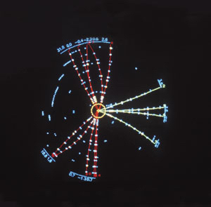
This same process does not only mean we had to compute some more to get a good estimate but it also offers another test of QCD. If the quark anti-quark and gluon are energetic enough and are produced at angles sufficiently large with respect to each other, we can reconstruct the kinematics of the partonic event. In this case hadronization will occur after the partons separate a distance of fm as it always does, but the hadrons produced out of each parton will travel roughly in the original direction. This means we can expect the hadrons to be found around a ‘cone’ with axis in the original parton direction and smaller radius (or more tightly packed hadrons) the larger the momentum. This bunch of localized hadrons we call a jet.
A pair production of quark anti-quark at sufficient energy will then produce a pair of jets, and the process in the LHS of fig. 13 with the emission of an energetic gluon will produce three jets. So far we had reviewed evidence for quarks inside the proton, found that the ratio pointed at 3 colours but now if we find 3 jet events it will give evidence for the Gluon and an estimate of the coupling or dynamics, .
Three jet events were observed at PETRA as the one on the RHS of fig. 13 and the rate of this events provided an estimate for the coupling in QCD in another milestone in the corroboration of our model of strong interactions.
Running coupling constants
In these lectures we should not step outside of tree level realm but we should be made aware that every process receives extra contributions from what is sometimes called radiative corrections, quantum corrections or in general loop corrections. Here we just want to review an important consequence of these loop effects, the running of coupling constants.
A force is produced by the exchange of a mediator so let us look at corrections of the gluon and photon propagators. Remember that what we call tree level processes have all internal line momenta fixed by 4-momentum conservation to be linear combinations of in and out states momenta. At this level the propagator of a gauge boson diagrammatically is just a wavy line from one point to another. At the one loop level, with the interactions of QED and QCD, i.e. three point (matter-matter-gauge boson) and in the case of QCD also (gauge boson) and (gauge boson) we can build the diagrams in fig. 1477 7 There is one missing diagram for QCD, can you draw it? [Hint there’s a 4 gluon vertex in QCD]. In these diagrams the momenta of the propagator is not fixed by 4 momentum conservation, if they have momenta and the external momenta is we have , and , which we can solve with and with arbitrary loop momenta . This momenta we integrate over, with the two propagators we have something like;
| (7.7) |
This integral we won’t do but we note that for very large it goes as and will produce a logarithm (divergent actually). To make sense of this contribution we have to renormalise our theory (i.e. make sure that in the S matrix decomposition the stays a ) but after the dust settles and we get the final result what this divergence is doing is to remind us that we have to input the parameters of our theory at a certain scale . Explicitly we have with :
| (7.8) |
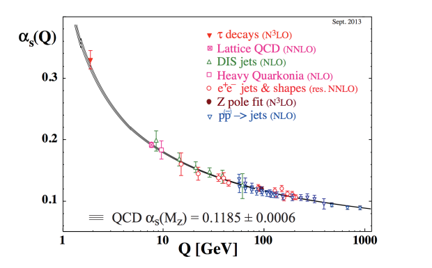
where is called the beta function and encodes the particulars of our theory, for QED and QCD we have
| (7.9) |
where is the number of quarks. The beta function in QED is negative, which back into eq. 7.8 means that for higher energy, , the coupling grows larger, . QCD on the other hand has the extra contribution, the ‘11’, which comes from the gluon diagrams and given that () we have . Therefore the non-abelian character of QCD makes it get weaker with higher energy. This is what we call asymptotic freedom and the reason we can trust partonic computations with quarks and gluons for high enough energy in QCD. You can see a plot of how the QCD coupling changes in fig. 15.
8 Electroweak interactions
The most prominent feature of the electroweak interactions is that the gauge symmetry is hidden at low energies. Not all of it however, out of the ‘breaking’ a part of if comes out intact, and that is electromagnetism. This lecture will work out how this comes about and the consequences of the breaking.
As we understand it nowadays, the vacuum expectation value (vev) of the scalar in our matter content is non-zero. In particular
| (8.1) |
with GeV. This is actually not hard to explain with the potential we wrote
| (8.2) |
so the configuration that minimizes the energy is that for which
| (8.3) |
where we note that we are assuming otherwise the minimum will sit at and there would be no electroweak symmetry breaking (and the world would have looked very different for example hydrogen does not form for massless electrons).
With this much input one can now look at the consequences by simply going around the Lagrangian for the Standard Model and substituting the Higgs doublet for its vacuum value, in eq. 8.1.
Masses for gauge bosons
We look at the gauge sector first. Gauge bosons will get a mass which will come out of simply substituting the vev in . First let us do
then the kinetic term for the vev of the Higgs is just the modulus of this 2-vector as:
| (8.4) |
It is customary to define complex bosons as
| (8.5) |
Whereas we note that only the combination of bosons appears in eq. 8.4, so let’s give it a name:
| (8.6) | ||||
where we have defined both and the weak angle , . All these definitions back88 8 Can you derive this yourself? You’ll need ’s definition. into eq. 8.4
| (8.7) |
comparing with mass terms for vector bosons in the Lagrangian
| (8.8) |
one can extract the expression for the masses
| (8.9) |
How about the other gauge boson out of the 4 in ? With our definition of comes the orthogonal combination
| (8.10) |
which we can invert and use to substitute everywhere we find a , for , . In particular they show up in covariant derivatives so we can write with generality
| (8.11) |
where is short for and we have used the definition of the weak angle99 9 Can you derive line 3 from 2 in 8.11? You’ll need ’s definition. and are ladder operators , . With this expression for covariant derivative in terms of mass states , , we can recast the field strengths and their squares in the Lagrangian and . One can use the relation
| (8.12) |
to find and in terms of using eq. 8.11. The fact that we define our mass states with an orthogonal definition (eq. 8.10) means they will stay cannonically normalized, but in addition the non-abelian character of will bring vector boson self interactions like those in fig. 16. In these lectures we won’t derive their form but note that the photon couples to the linearly as it should cause the is charged.
We turn next to the coupling of electro-weak bosons to fermions. The electromagnetic coupling is defined as and the combination in the last line of eq. 8.11 should give us the charge for each field, let’s see
| (8.13) |
| ( , ) | ( , ) |
where we have used chiral projectors to condensate notation.
You can amuse yourself to fill up table 17 and find that this actually gives the charges we know of, e.g
In particular electromagnetism is not chiral, which means and no in the coupling of the photon to fermions. For the and bosons however the chiral nature of the Standard Model will leave an imprint. This is clearest in the interactions of the W boson which only couples to left-handed fields. To interpret what these types of couplings imply we turn to chirality next.
Chirality
Chirality and handedness is not a good quantum number for Dirac fermions, that is, they are not in a specific chirality state but rather a superposition. The reason for this is that a Dirac mass term mixes left and right fields. This we can see explicitly in the SM after substitution of in the Yukawa couplings
| (8.14) | ||||
| (8.15) |
and so we have that the Higgs also gives masses to the fermions with . The exception are neutrinos which are massless in the SM (but not in nature).
One has nonetheless that in situations in which the mass of the fermion can be neglected, chirality does have a simple physical interpretation, it’s helicity:
with helicity being spin projection on the three-momenta direction. In this way the couples to helicity neutrinos and as for helicity neutrinos we do not even know if they exist because is a different field !
Let’s use neutrinos to exemplify how chiral interactions couple differently to spin and violate parity in the process.
Assume we can prepare a boson with spin in the direction and assume it decays into positron and a neutrino traveling in the original spin direction, and in a given helicity state. Momentum conservation fixes the spins of the two fermions to be aligned in the direction which, depending on which way the neutrino is going, means different helicity.
Let’s first take the neutrino going backwards, then it has helicity and we have a LH neutrino. The neutrino going the other way we can obtain with a parity transformation, parity flips sign in and hence but spin has two components and doesn’t flip. In resume (parity)()=() whereas for spin (parity) and helicity (parity)=. This is easier to sketch than to say, and so does fig. 18. The parity transformation brings us then to a helicity neutrino and such a particle (if it exists) does not couple to the boson. So we have that weak interactions distinguish helicities and violate parity; positrons are only shot forwards!.
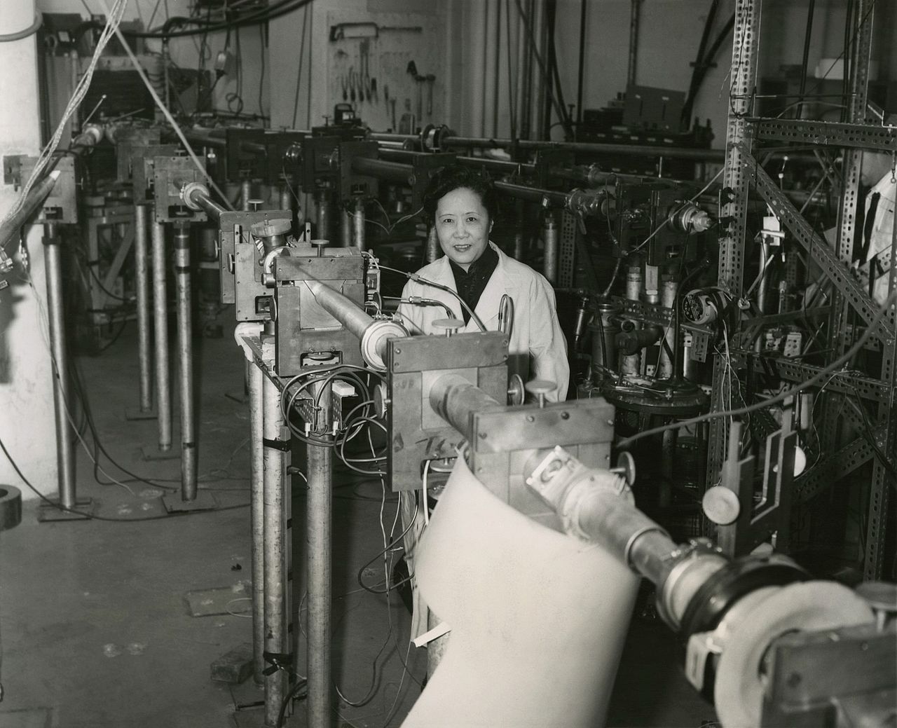
Although this was an idealized scenario, it translates to more realistic ones mediated by the weak interaction. As a relevant example Chien-Shiung Wu showed experimentally that in the decay of polarized Co to Ni and an electron and anti-neutrino, the electrons were only going one way. This discovery lead to Tsung-Dao Lee and Chen-Ning Yang winning the 1957 Nobel prize in physics while she was awarded the first Wolf prize in 1978.
Z,W couplings to fermions
One has then that the charged boson retain the left handed character of the group, while for the boson we rewrite the covariant derivative, using the projectors, as
| (8.16) | ||||
where we have used the relations for in eq. 8.13 to substitute hypercharges and . We see then that the boson retains part of the left-handedness but also has a vector coupling proportional to the electromagnetic charge of the given fermion. Before moving on let us put this covariant derivative in the action for quarks to write explicitly:
| (8.17) |
So finally we have written interactions in terms of mass eigenstates , which are the ones we see in experiment, starting from the original gauge bosons . The pattern of breaking can then be summarized as and leaves behind massive , bosons which we cannot produce at low energies where we only ‘see’ the familiar photon with the charges that derive from a combination of hypercharge and weak isospin.
9 Elecroweak Bosons properties
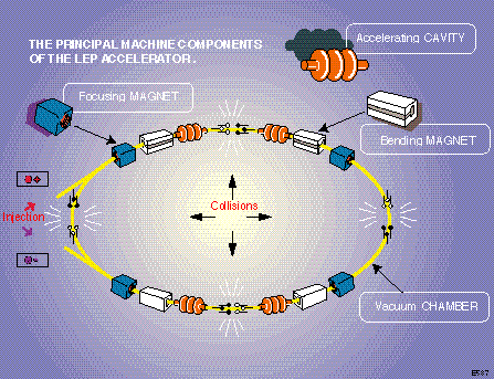
Discovery of the bosons, theorised in the 60s, had to wait till the 80’s and the Super Proton Synchrotron (SPS) at CERN. The SPS is a synchrotron accelerator with 6.9km of circumference and capacity to accelerate protons anti-protons electrons positrons. For the discovery of the electroweak bosons it operated as a proton-antiproton collider for the UA1 and UA2 detectors. In order to study the properties to an accuracy of permile level, the SPS was used as an injector for a bigger collider, the Large Electron-Positron collider (LEP).
|
|
Electron and positrons accelerated at the SPS were later transferred to LEP in a 27 km circular tunnel (which nowadays hosts the LHC) and were accelerated to initially GeV (GeV) and in a second stage to GeV (GeV).
From the covariant derivative we derived in eq. 8.16 we see that the couples to the electron field with an interaction that could mediate electron-positron annihilation into a boson. Consider for example a process like which has an invariant matrix element
| (9.1) |
with . As mentioned above LEP initially ran at where the propagator in the formula above seemingly blows up! Indeed when the particle is produced on resonance () one has to reconsider the process at hand. In this regime the particle is no longer virtual but the centre of mass energy is just right to produce it. If the particle were stable, this ‘blowing up’ or discontinuity of the amplitude would be telling us that is itself a possible process on its own and can be a final state. If instead the particle is unstable, and in particular with a a short lifetime so that it decays within our experiment one has to modify the particle propagator, which is to say how the particle evolves with time.
The easiest way to do this from the formula above is to substitute the mass in the denominator as with the total decay width of the boson (the decay width is the inverse of the lifetime ). This extra imaginary part in the action for the particle gives a time evolution for the wave-function, in the rest frame, as and hence the probability (—wavefunction—) decays exponentially as . The resulting propagator and cross section will scale as
| (9.2) |
This is called a Breit-Wigner distribution and looks like a peak at sharper the smaller . In the jargon of particle physics we call small a narrow resonance and large a broad resonance.
In the case of a well defined peak () the narrow width approximation applies and we can compute the cross section as the exchange of an on-shell which implies production and decay are factorized1010 10 This is true when one computes total cross sections integrating over angles and averaging over spins, if one considers differential rates some entanglement of initial and final states remains. which reads for the cross section
| (9.3) |
This allows for the computation to be broken down into smaller pieces and for our experiment to look for all different decays and reconstruct the couplings of the boson. Let us focus on one in particular for a sample computation, and the decay . The interaction term we can derive from the original Standard Model Lagrangian by focusing on the neutrino field in the lepton doublet and it reads
| (9.4) | ||||
| (9.5) |
so for neutrinos we have that the boson preserves the chiral character of and couples only to LH fields. This is also one of the reasons why we have no evidence of RH neutrinos since as we will see the couples as well to LH fields and neutrinos have no other known interactions. The invariant matrix element is
| (9.6) |
If we are computing the rate we average over initial states which could be any of the three polarizations and we sum over all possible final states, that is:
| (9.7) | ||||
| (9.8) | ||||
| (9.9) |
we now use the fact that we can bring one towards the other and and then1111 11 the relation
| (9.10) |
to find
| (9.11) | ||||
| (9.12) |
where given that is fully antisymmetric the contraction with the averaged cancels.
Now let us work on the phase space and the invariant contraction of momenta, for simplicity we sit on the CM frame
| (9.13) |
this also means that the functions of momenta in the invariant matrix element squared read:
| (9.14) |
where we have used 4 momentum conservation and in particular the fact that neutrinos share the mass, . Finally, all together:
| (9.15) | ||||
| (9.16) |
| (GeV) | (GeV) |
|---|---|
| decay products | |
| invisible | |
| hadrons |
One last thing we forgot is, how many neutrinos are there? Say , then
| (9.17) |
One can then compare with experiment to test the theory. As it turns out we did not pick an observable easy to extract from experiment; neutrinos escape the detector unseen. There is a way to get around this however; from a cross section plot like in fig. 20 one can extract the total width . Then from the visible Z decays we can reconstruct partial widths to charged leptons, hadrons; the difference between the total and the sum of all this visible channels must be neutrinos, or as commonly refereed to, invisible. One can then contrast this difference with eq. 9.17 and, provided we know and , determine . What one finds is
| (9.18) |
which is a pretty good ‘determination’ of the number 3.
| (GeV) | (GeV) |
|---|---|
| decay products | |
| hadrons |
You can see a summary of the boson properties as extract from LEP in fig 22 and in particular the different branching ratios or how likely is the boson to decay to the given final state. For completeness the properties of the charged boson are given in table 23. The boson cannot be produced like the boson, that is ‘in the s channel’ of collisions but one can produce pairs via for example or also via the boson itself . The condition for this to occur is having a center of mass energy high enough, i.e. as we had in the second run of LEP. Not listed here but of relevance are angular-dependence studies of decays which offer light on the chiral structure of the couplings (you will get to see it in the workshops).
Finally one other prediction of the SM is the ratio of masses for ,. If one independently determines from for example and the electromagnetic coupling constant with the values of masses we can construct a ratio which is predicted to be in the Standard Model. This ratio is found to be experimentally,
| (9.19) |
In another confirmation of the Standard Model of particle physics.
10 The Higgs boson
The Higgs boson corresponds to the radial component of the potential in 8. As opposed to the angular component along which one can move at no cost in energy, the radial direction has curvature. This means that when we expand around the vacuum the potential has
| (10.1) | ||||||
where given that , the term linear in cancels. The next term, , associated with the curvature at the minimum, will produce a mass for the Higgs. We now know this mass to be GeV1212 12 Note that this is not ; the curvature at the local maximum () and minimum () are different. Can you figure out the connection ?.
To find how this boson couples to matter we can do the same as we did to observe electroweak-symmetry breaking in 8 in play and substitute as in equation 10.1 in our Lagrangian. Instead of doing this all over again, a shortcut is simply to take the formulas we obtained and substitute . This means that the Higgs will couple proportionally to elementary particle masses, with propotionality constant . Let us then write the linear couplings of the Higgs at tree level
| (10.2) | ||||
| (10.3) |
where we omit higher powers of , i.e. One can translate the above Lagrangian into Feynman rules for the vertexes as
Rather than me telling you once more let’s try to figure out how the discovery of this particle came about in terms of Feynman diagrams. As you might know, LHC collides protons against protons, which in terms of the initial elementary particle states means we have quarks, antiquarks and gluons at our disposal. So the problem we lay out first is how to produce a Higgs particle from these states, something like we have in fig. 24. There might be different ways to produce a Higgs and it might come with extra particles, but among all these possibilities we are interested in those which are the most likely. For this we should focus on what does the Higgs couple more strongly to. The process need not even be a tree-level process, one loop level processes have an extra (coupling) suppression, for your estimates. One final consideration is how much of each inital state is there in the proton, an information contained in the parton distribution functions. I don’t expect you know these quantitatively so take a guess from their shape.
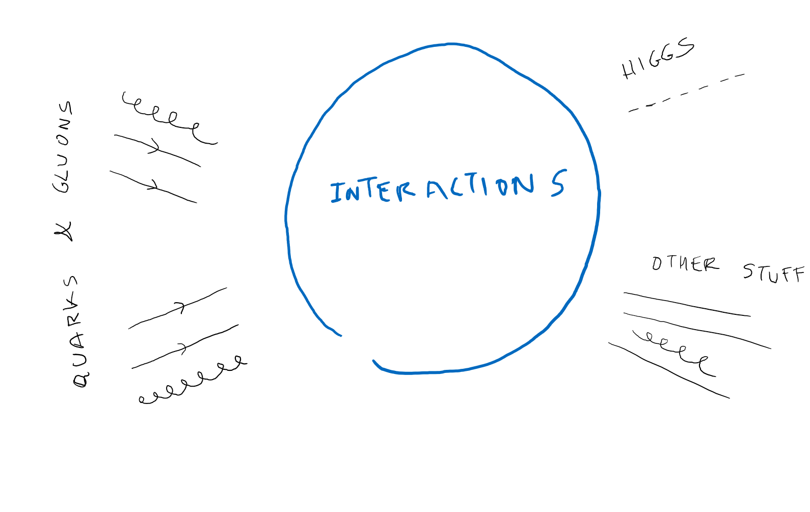
Okay so give yourself some time and draw diagrams which you think can do the job, not writing the matrix element. Put in just for an estimate though the couplings involved, , . When you think you’re ready turn the page to find the answer.
Higgs production
Although there are quarks and antiquarks in the proton, they are predominantly the first few generations and they couple very weakly to the Higgs due to their light masses, e.g. . What happens more often is that a quark anti-quark annihilate into a vector boson, to which they couple with strength and then this electroweak boson emits a Higgs, this is called Higgstralung or vector boson associative production and is diagram (c). One can have instead, using the same vertexes, two vector bosons emitted from quarks or antiquarks, which increases the number of contributing initial states, annihilating into a Higgs. This process has one more coupling w.r.t. to the previous but this is made up for in density of initial states so that this is a more probable production mechanism. This is shown below, (b) and is called vector boson fusion.
|
|
|
|
|
Another initial state available in abundance are gluons which however are massless and do not couple directly to the Higgs. They do couple to the top, and this is the particle that couples the strongest to the Higgs with .
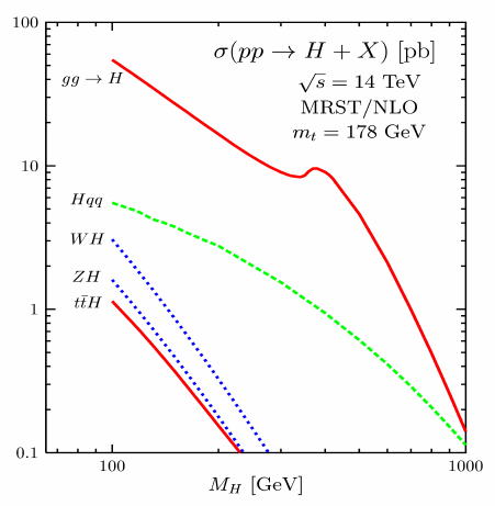
One can then have two gluons producing a top anti-top pair out of which a Higgs is emitted. This comes at a higher energy cost since we have to produce not only the Higgs which ‘costs’ but also the top pair which requires an extra GeV. This is called associative production and is diagram . Finally we can avoid having tops in the final state if we have them annihilate back after they emit the Higgs. This implies a closed fermionic line and it is a loop process, compared to the previous gives an extra factor . This nonetheless is made up for in phase space and pdfs and this process (a) is called gluon fusion. The cross sections for each of this processes can be seen in fig. 25.
Next it’s Higgs decay. Try sketch diagrams for its decay before turning the page.
Higgs decay
The diagrams for Higgs production do actually give a good idea of how could it decay by just turning back time.
|
|
|
The main difference is however that for the Higgs to decay to a given state there must be enough phase space or in simpler terms enough energy. This precludes decays to the particles that couple the strongest to the Higgs, that is which require respectively some , & GeV. Next in line therefore are b quarks, whose coupling is considerably small but given the Higgs mass of 125 is the main decay mode (a). It is followed by the decay into a and a pair of fermions via a virtual , like we said we cannot have the decay
|
|
|
|
to two ’s but given the strength of the coupling to weak bosons this second order in decay is the second source in relevance (b). Note that in fig. 26 the mode means actually for . Next is the inverse of Gluon fusion, which is and is a loop process with virtual tops which would be observed as two jets in the detector (c).
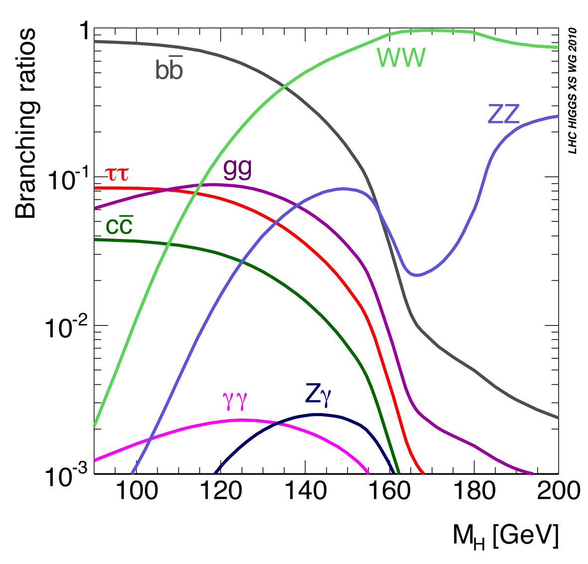
This is followed by and , . Finally, although much less likely, the Higgs can decay to two photons () (d) via the loop diagram similar to gluon fusion but now with tops and in the loop (the eletromagnetically charged particles that couple the strongest to ) or Higgs to photon (). These decays leave a clear signal in the detector and were an essential part of the Higgs discovery.
The respective branching ratios are shown in figure 26. Note that given the Higgs mass we have predictions for all of them so we can test once more the SM against data. At present the couplings agree with the SM but the experimental precision is at the 10% level.
11 Flavour
In this lecture we will outline the flavour structure and phenomenology of the Standard Model. For a while now we have been setting the flavour structure aside, either focusing on the first family or ‘hiding’ flavour indices which are summed over, e.g. when we say the down-type quarks couple to the photon as we mean all of them couple the same with a sum on and . Indeed, as far as the photon is concerned, all down-type are the same. The one property that allows us to distinguish between them is their mass, and as we have seen mass comes from the coupling to the the Higgs, the Yukawas:
| (11.1) | ||||
| (11.2) |
where in the second line we restored matrix notation and the mass matrices are . In this language, the Yukawa couplings are a complex matrix for each up, down and lepton type. One has that any complex matrix can be diagonalized by a unitary rotation from the left and one from the right. That means
| (11.3) | ||||||||
with unitary . The masses are displayed in fig. 27, as you can see, the spread in masses over many orders of magnitude means the entries of these diagonal matrices have a strong relative hierarchy.
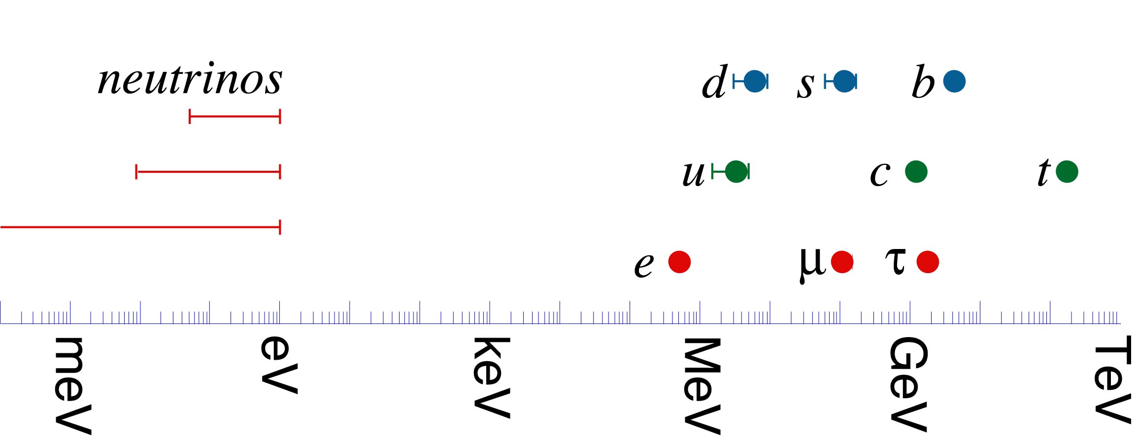
Just like we did for electro-weak gauge bosons we now rotate to the mass basis
| (11.4) |
and equivalently for the RH fields so that the mass terms originated from Yukawa interactions are diagonalized
| (11.5) |
What is important to realize now is which parts of our action ‘care’ about this rotation. As we said the only couplings that had flavour structure are the Yukawas (mass terms) which we diagonalize with the rotation above. Because the Higgs couples proportional to mass, this also means that the Higgs couplings will be diagonalized. The remaining couplings of fermions are then to gauge bosons.
In matrix notation, the couplings to e.g. the photon are proportional to the identity in flavour space which means that a unitary rotation of (and so ) leaves the couplings the same . The rotations however are chiral, different for LH and RH, does this argument still hold then?
Let’s take a general current and prove that it only couples LH to LH and RH to RH:
| (11.6) | ||||
where in the second line we used . All of the gauge boson couplings are of the form above, so it looks like the unitary rotations might cancel out. Just to make sure we look at the couplings and do it carefully
| (11.7) | ||||
| (11.8) |
Indeed the unitary rotations disappear. So would happen for the photon couplings, but we have that the case of the , which couples to different-charge fermions, is different,
| (11.9) |
Where we have defined the Cabibbo-Kobayashi-Maskawa and Pontecorvo-Maki-Nakagawa-Sakata unitary mixing matrices. For leptons we have not defined a mass term in the neutrino sector but we assume they have a mass1313 13 The neutrinos could be Dirac-like and have a mass or Majorana and have instead ; in both cases we would have to rotate the neutrinos by . and get rotated to the masss basis also. If we were to stick strictly to the Standard Model, neutrinos would be massless and we can choose to eliminate the mixing and restore lepton number conservation.
These couplings to the , if the mixing matrices have off-diagonal components, are the only place to ‘jump’ from one generation to another. Indeed the ‘charged currents’ or couplings to the are the source of decay of heavier generations to lighter ones. The shape of this mixing matrices we have determined experimentally although not in full yet for leptons.
The mixing matrix for quarks is close to the identity, and we can parametrize it with 4 variables and an expansion around 1 as
| (11.10) |
whereas on the other hand the mixing matrix for leptons has larger angles and it is not close to the identity. In this case it conventional to use Euler angles as
| (11.11) |
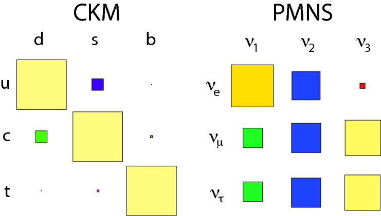
The presence of complex coefficients in these matrices signals CP violation, which has been observed in quarks () but not yet in leptons (). In addition if neutrinos are Majorana particles two extra Majorana phases appear, but this also is not known yet. The relative size of entries in these matrices is depicted in fig. 28. Together with fig. 27 this gives the flavour structure for the elementary particles, as to why it is what it is, it is an open question.
The fact that the only source of flavour or possible generational jump appears in couplings to the W boson is referred to as no flavour changing neutral currents (FCNC) at tree level. This has consequences for phenomenology since it means that certain decays are not allowed at tree level. For example occurs at tree level mediated by a charged current ().
On the other hand cannot ocur at tree level and the same goes for e.g. or . These processes occur at the one loop level as shown in fig. 29 and are mediated by the couplings and the mixing elements. This means that the invariant matrix elements for each process will scale with the mixing and masses of the internal particles as respectively
| (11.12) |
were I do not want you to take in the specifics but just the sense that, because of the loop suppression and small mixing elements (for quarks) and or small mass ratio (quarks and leptons) these effects are much more rare. Let me be clear, except for lepton flavour violation, they occur in the SM as opposed to e.g. baryon number violation, only not too frequently. Which also means these processes are good places to look for other physics beyond the Standard Model.
|
|
|
|
12 Beyond the Standard Model
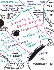
References
- [1] (2008) Introduction to elementary particles. External Links: ISBN 978-3-527-40601-2 Cited by: item [1].
- [2] (1984) QUARKS AND LEPTONS: AN INTRODUCTORY COURSE IN MODERN PARTICLE PHYSICS. External Links: ISBN 978-0-471-88741-6 Cited by: item [2], Figure 12.
- [3] (1955) On the formulation of quantized field theories. Nuovo Cim. 1, pp. 205–225. External Links: Document Cited by: §3.
- [4] (1995) An Introduction to quantum field theory. Addison-Wesley, Reading, USA. External Links: ISBN 978-0-201-50397-5 Cited by: §3.
- [5] (2013) Modern particle physics. Cambridge University Press. External Links: Document Cited by: item [5].
- [6] (2011) Elementary particle physics in a nutshell. Cited by: item [6].