PHYS3621 Foundations of Physics 3a
Nuclear Physics

What are the most elemental components of matter? Our answer to this question has been evolving with time as our knowledge progressed finding appropriate descriptions at each increasingly small scale. Here we zoom in to femto-metre (fm) distances to explore nuclear structure; the forces, the components and the conservation laws that rule over this sub-atomic world. We will develop the formalism in quantum mechanics and special relativity that allows us to look deep into matter, learn about nuclear binding energies and transitions, and the models that help us understand them.

1 Introduction and units

These notes contain an introduction to nuclear physics, but how is nuclear physics relevant to us? In our everyday macroscopic life the inner workings of the nucleus of atoms have seemingly little consequence. Gravity bounds us to earth, electromagnetism rules the flow of electrons that power our appliances and the propagation of the few-hundred-nanometre wavelength field through which we see our world; the role of nuclear forces is to hold the positively charged component of the atom together, what could we possibly gain from studying it? Well, a source of energy that supplies a sixth of the consumption in the UK, a gateway to the more elemental description of nature that is Quantum Chromo-Dynamics and an understanding of the range of chemical elements that make up our universe and allow for carbon-based life forms to ask the question in the first place.

There seems to be then some motivation to learn about nuclear physics, but how do we ‘look’ into this sub-atomic world? We can only ‘see’ so far in the conventional sense; optical microscopes resolve distances down to $\sim 100$ nm. This limitation comes from the medium we use to see itself; we cannot resolve details smaller the wavelength, $\lambda$, of the medium we are using (you might have encountered this in solid state physics, looking at a crystal with the naked eye you see a block, shine X-rays and you’ll be able to resolve the crystal structure from diffraction patterns). Electron microscopes can zoom in 3 orders of magnitude more to $100$ pm, their resolution given again by wavelength, now estimated from the momentum as:

$\lambda$ $={\displaystyle \frac{h}{p}}$ $h$ $=6.626\times {10}^{-34}{\text{kg m}}^2{\text{s}}^{-1}$ (1.1)

where $h$ is Planck constant and this is de Broglie’s equation which puts on the same footing photons and electrons through quantum mechanics. It also tells us that if we want a smaller resolution we have to increase the momentum and with it, the energy. If we keep increasing the energy we have that our probe into the subject of study might change it. In this case we end up with a collision or scattering experiment where the initial and final states are different. This type of experiment requires analysis; we are no longer taking ‘photos’ that we can look at and immediately comprehend, we should look at it through the lens of quantum mechanics.

This is indeed the way we did probe the smallest scales known to date, not only in nuclear physics but also in particle physics, descending to scales a thousand times smaller than a nucleon. Let’s introduce then the basic elements of scattering experiments.

1.1 Scattering experiments

Consider a stream of particles directed to a target. The target has a characteristic area for interaction with the incident particles; in classical mechanics and for neutral objects this is the area of our object projected on the direction of the incoming projectiles e.g. $\pi R^2$ for a billiard ball of radius $R$. In general this area can be larger than the target size and we call it cross section, denote it $\sigma$ and measure it in units of barn (b) with 1b$={10}^{-28}$ m${}^2$.

To estimate how many of the incident particles will get deflected or scattered one has to calculate how many of them pass through the area $\sigma$ around the target. More projectile particles, more tightly packed or faster will result in more scatterings events; this is characterized by the flux of particles

$$\text{ Flux}=\frac{\text{Number of incoming particles}}{\text{ (Area) }\times (\text{ time})}=\frac{N_{in}}{A\times t}\equiv F$$

The number of deflections in a given time interval $\mathrm{\Delta }t$ is then

Flux= $Ni⁢nA⋅t     σ$ (1.2)

$$N_{\text{ scat}}=\frac{\text{ Number of incident particles}}{\text{ (Area) }\times (\text{ time})}\times \text{cross section}\times \text{ time interval }=F\times \sigma \times \mathrm{\Delta }t$$

If you want to make sense of this formula in more familiar terms think of how many drops of water would fall in your $\sim 0.5$m${}^2$ umbrella in 5 min if it rains with a flux of 12 drops per squared metre per second.

In practice our experiments have many targets to increase the observed dataset, in this case one just sums over all targets, assuming they all see the same flux:

$$\frac{N_{\text{scat}}}{\mathrm{\Delta }t}=F\times N_{\text{targ}}\times \sigma \equiv ℒ\times \sigma$$

Where we have defined the luminosity $ℒ$ which is the generalization of flux for scattering experiments, is measure in inverse barn per second b${}^{-1}$ s${}^{-1}$ and gives us the number of events per unit time when multiplied by the cross section.

Whereas the luminosity characterizes our experiment, cross section can a priori be computed from first principles which is what allows for testing our theories of Nature against Nature itself.

1.2 Natural units

In nuclear and specially in particle physics natural units are frequently used. In practice natural units are not just just another system but it also involves a prescription. The reason for adopting this system is measuring quantities in units given by the fundamental constants of nature, two in particular

$$\cdot \text{speed of light }c\mathit{\hspace{1em}\hspace{1em}\hspace{1em}\hspace{1em}}\cdot \text{Planck’s reduced constant }\mathrm{\hslash }=h/(2\pi )$$

So in these units a car travels at $0.0000001$ c or an Olympian reaches ${10}^{35}\mathrm{\hslash }$ in hammer throw but an alpha particle from radioactive decay might have $0.01$ c and an electron has spin $\mathrm{\hslash }/2$. What makes natural units less straightforward than other units is that one also omits c and $\mathrm{\hslash }$. Making them implicit has the advantage of simplifying our computations, since in practice it means

Natural units $c$ $=1$ $\mathrm{\hslash }$ $=1$ (1.3)

So some of the equations you know simplify:

$i\mathrm{\hslash }{\displaystyle \frac{\partial }{\partial t}}|\mathrm{\Psi }⟩$ $=E|\mathrm{\Psi }⟩$ $\mathrm{\Delta }p\mathrm{\Delta }x$ $\ge {\displaystyle \frac{\mathrm{\hslash }}{2}}$ $E$ $=m{c}^2$ (1.4)

$i{\displaystyle \frac{\partial }{\partial t}}|\mathrm{\Psi }⟩$ $=E|\mathrm{\Psi }⟩$ $\mathrm{\Delta }p\mathrm{\Delta }x$ $\ge {\displaystyle \frac{1}{2}}$ $E$ $=m$ (1.5)

From these equations one can also deduce that the units of time, space, mass and momentum are all related to those of energy in natural units as

$[t]=$ ${[E]}^{-1}$ $[m]$ $=[E]$ $[x]$ $={[E]}^{-1}$ $[p]$ $=[E]$ (1.6)

The choice for energy in natural units is electronvolt (eV) and time, space, momentum and mass are given as powers of this basic unit.

In summary, if somebody gives you speed or angular momentum in natural units, multiply by c or $\mathrm{\hslash }$ respectively to convert to other system and for time, space, mass or a composite of these use powers of $\mathrm{\hslash }$, c as in table 1.

Magnitude	S.I.	N.U.	conversion
Speed	m/s		(N.U.)$\times$ c $=$ (N.U.)$\mathrm{\hspace{0.17em}\hspace{0.17em}3.00}\cdot {10}^8$m s${}^{-1}$
Angular momentum	J s		(N.U.)$\times \mathrm{\hslash }=$ (N.U.)$\mathrm{\hspace{0.17em}\hspace{0.17em}1.05}\times {10}^{-34}$ J s
Energy	J	eV	(N.U./eV) eV$=$ (N.U.)$\mathrm{\hspace{0.17em}\hspace{0.17em}1.60}\times {10}^{-19}$J eV${}^{-1}$
Mass	kg	eV	(N.U./eV) eV c${}^{-2}=$(N.U.) $1.78\times {10}^{-36}$kg eV${}^{-1}$
Distance	m	eV${}^{-1}$	(N.U. eV) $\mathrm{\hslash }$ c eV${}^{-1}=$ (N.U.)$\mathrm{\hspace{0.17em}197}$ fm MeV
Time	s	eV${}^{-1}$	(N.U. eV) $\mathrm{\hslash }$ eV${}^{-1}=$  (N.U.) $6.58\times {10}^{-16}$ eV s

Figure 1: Conversion between N.U. and S.I.

As an example a length $L$ of 0.005 eV${}^{-1}$ in N.U. is

$\text{N.U.}\mathit{\hspace{1em}}L$ $=5\times {10}^{-3}{\text{eV}}^{-1}$ $\text{S.I.}\mathit{\hspace{1em}}L\times 197\text{MeV fm}$ $\simeq \text{ nm}$ (1.7)

A useful reference for fundamental constants and conversion factors is the p.d.g.

2 Relativistic Kinematics

The relation between energy and mass for a particle at rest is one of the most publicized equations in science and here we will find use for it. First however, the actual relation for a particle with speed $v$ is:

$E={\displaystyle \frac{m{c}^2}{\sqrt{1-{(v/c)}^2}}}={\displaystyle \frac{m}{\sqrt{1-v^2}}}$ (2.1)

where the second line is in natural units. A small velocity expansion returns the familiar kinetic energy (it is a good exercise to do this explicitly). This equation also tells us that the energy is different for different observers, in particular higher the larger relative speed and always larger than the energy in the rest frame. Similarly, although not evidently so, an event with a given duration on its rest frame will appear to last longer for another observer. This time dilation is the same factor as the ratio of the energy and mass, let’s see why.

This observation follows from special relativity, which in its rather minimal formulation, groups together different magnitudes together in 4-vectors. These four-vectors are represented by a letter with an index which in our convention will be a Greek letter

$x^{\mu }$ $=\left(\begin{array}{c}\hfill t\hfill \\ \hfill x\hfill \\ \hfill y\hfill \\ \hfill z\hfill \end{array}\right)=\left(\begin{array}{c}\hfill t\hfill \\ \hfill 𝐱\hfill \end{array}\right),$ $p^{\mu }=$ $\left(\begin{array}{c}\hfill E\hfill \\ \hfill p_x\hfill \\ \hfill p_y\hfill \\ \hfill p_z\hfill \end{array}\right)=\left(\begin{array}{c}\hfill E\hfill \\ \hfill 𝐩\hfill \end{array}\right).$ (2.2)

The reason this is not a purely aesthetical arrangement is that magnitudes within a four-vector get mixed up for different observers.

Consider this situation, you are sitting down in your frame with coordinates $x^{\mu }$ and an observer ${𝒪}^{\prime }$ moving at a relative speed $v$ ($\beta =v/c$) along the x axis and towards $x=\mathrm{\infty }$ passes you by at $t=0$. Her/his coordinates are $x^{\prime \mu }$, to translate them into yours we do

$\gamma$ $={\displaystyle \frac{1}{\sqrt{1-{\beta }^2}}}$ (2.3)

This means that an event at rest in the original frame which takes $t_e^{\prime }$ seconds, i.e. $x_e^{\prime \mu }=(t_e^{\prime },0,0,0)$, seems to take $t_e=\gamma t_e^{\prime }$ for you, that is it takes a factor $\gamma$ longer. Equivalently a particle at rest for ${𝒪}^{\prime }$ has energy $m$ and no momentum, $p^{\prime \mu }=(m,0,0,0)$, whereas you measure a 4-momentum

$$p^{\mu }={(\gamma m,v\gamma m,0,0)}^T$$

and we recover the expression for the energy 2.1. The non-relativistic limit gives us the usual expression for momentum and energy but we see here that it breaks down when velocities are close to c and $(\gamma -1)\sim 1$.

In our scattering experiments we express kinematics in terms of 3-momentum $𝐩$ rather than speed; according to our derivation the connection is $𝐩=\gamma m𝐯$, but then how do we write the energy in terms of momentum? Direct substitution would do it but here let us instead use the invariant scalar product of a four vector, defined as

$p^2\equiv$ $p^{\mu }{\eta }_{\mu \nu }{p}^{\nu }=p_{\mu }{p}^{\mu }=p^{\mu }{p}_{\mu }=E^2-{𝐩}^2$ ${\eta }_{\mu \nu }$ (2.4)

where we used Einstein’s convention i.e. repeated indexes are summed over. The use of this scalar product is that every observer will measure the same magnitude and the simplest frame to compute it is the particle’s rest frame where ${(p^{\prime })}^2={(p_0^{\prime })}^2=m^2$, but we can explicitly check that we get the same in our frame

$p^2=$ ${\gamma }^2(1-v^2)m^2=m^2\stackrel{(\mathit{\text{<a href="\#S2.E4" title="(2.4) ‣ 2 Relativistic Kinematics ‣ PHYS3621 Foundations of Physics 3a Nuclear Physics" class="ltx\_ref ltx\_font\_italic" style="font-size:70\%;"><span class="ltx\_text ltx\_ref\_tag">2.4</span></a>}})}{=}{E}^2-{𝐩}^2$ $E=\sqrt{m^2+{𝐩}^2},\boxed{𝐯={\displaystyle \frac{𝐩}{E}}}.$ (2.5)

This is the relation between momentum and energy that we will employ in the following.

The grouping of energy and momentum into a 4-vector also makes the conservation laws for energy and momentum more compact. Take for example a particle with momentum $p$ decaying to two particles A and B with momentum $k_A$, $k_B$. We have

$$p^{\mu }=k_A^{\mu }+k_B^{\mu }$$

If we take the square on both sides we will obtain an invariant magnitude as:

$$m^2=m_A^2+m_B^2+2k_A\cdot k_B\mathit{\hspace{1em}\hspace{1em}\hspace{1em}\hspace{1em}\hspace{1em}}{k}_A\cdot k_B=\frac{m^2-m_A^2-m_B^2}{2}$$

which is the same quantity in all frames; that is, take the energy of particle A times the energy of particle 2, subtract the product of their 3-momenta and the magnitude you get is, regardless of your relative velocity, $(m^2-m_A^2-m_B^2)/2$.

3 Scattering from Fermi’s Golden rule

The number of scattering events in our experiments is given by luminosity $ℒ$ (flux times number of targets) and cross section $\sigma$. We have control over $ℒ$ since we can tune it as part of our initial state preparation, $\sigma$ on the other hand is a fundamental property of our particles which we can compute from theory. This means that, given a theory, one can predict the number of scatterings & then confront this prediction against the outcome of the experiment to prove or disprove our ideas. In this chapter we turn to how we compute this cross section.

To make this computation we will $(i)$ introduce momentum eigenstates in the continuum to describe our initial and final states and $(ii)$ use perturbation theory (Fermi’s Golden rule) to calculate the probability for scattering $(iii)$ compare with our expression for number of scatterings. For another derivation of these results see [1].

3.1 Momentum eigenstates

Let us start the computation in a box of side $L$ and volume $V=L^3$. We set periodic boundary conditions for our wave-function at the edge of the box. This discretizes the momentum states since we can only fit integer multiples of the wavelength, that is

$p_x=$ ${\displaystyle \frac{h}{{\lambda }_x}}={\displaystyle \frac{2\pi \mathrm{\hslash }}{L/n_x}}={\displaystyle \frac{2\pi }{L}}{n}_x$ (3.1)

where in the last line we used N.U. and we note that our spacing in momentum is $\delta p=2\pi /L$. Momentum is however not discretized in our scattering experiments which can be understood as taking the large volume limit which yields a continuum spectrum. However in taking this limit we should take care in particular to define our sums over states, in particular inverting the above our sum over momentum states looks like

$n_x$ $={\displaystyle \frac{L{p}_x}{2\pi }}$ ${\displaystyle \sum _{n_{x,y,z}}}\to$ ${\displaystyle \int d^{3}n}={\displaystyle \int \frac{V}{{(2\pi )}^3}{d}^{3}p}$ (3.2)

On the other hand we can write the wave function for our states as

${\mathrm{\Psi }}_{𝐩}(𝐱)=$ $⟨𝐱|{\mathrm{\Psi }}_{𝐩}⟩={\displaystyle \frac{e^{i𝐩\cdot 𝐱}}{\sqrt{V}}}$ ${\displaystyle {\int }_V}𝑑x^3$ ${|{\mathrm{\Psi }}_{𝐩}(𝐱)|}^2=1$ (3.3)

Our momentum states however should not depend on volume which will be set to infinity so we define them as

$|{\mathrm{\Psi }}_{𝐩}⟩\equiv {\displaystyle \frac{|𝐩⟩}{\sqrt{V}}}$ $⟨𝐱|𝐩⟩$ $=e^{i𝐩\cdot 𝐱}$ (3.4)

3.2 Fermi’s Golden rule

You have seen Fermi’s Golden rule in the first part of this module for an oscillating perturbation. Here our perturbation or interacting Hamiltonian will be time independent which makes the derivation somewhat simpler. As usual we split our Hamiltonian into a free and an interacting term

$i{\displaystyle \frac{\partial }{\partial t}}|\mathrm{\Psi }(t)⟩$ $=\left({\mathscr{H}}_0+{\mathscr{H}}_{\text{int}}\right)|\mathrm{\Psi }(t)⟩$ ${\mathscr{H}}_0|{\mathrm{\Psi }}_{𝐩}⟩$ $=E_{𝐩}|{\mathrm{\Psi }}_{𝐩}⟩$ (3.5)

Note that $|𝐩⟩$ is also an eigenstate of ${\mathscr{H}}_0$ since it is only differs from $|{\mathrm{\Psi }}_{𝐩}⟩$ by a scaling factor. The solution to Schrodinger’s equation is then, in matrix notation

$e^{i{\mathscr{H}}_{0}t}|\mathrm{\Psi }(t)⟩=$ $\text{Exp}\left(-i{\displaystyle {\int }_0^t}𝑑t^{\prime }{e}^{i{\mathscr{H}}_0{t}^{\prime }}{\mathscr{H}}_{\text{int}}{e}^{-i{\mathscr{H}}_0{t}^{\prime }}\right)|\mathrm{\Psi }(0)⟩$ (3.6)

$\simeq$ $|\mathrm{\Psi }(0)⟩-i{\displaystyle {\int }_0^t}𝑑t^{\prime }{e}^{i{\mathscr{H}}_0{t}^{\prime }}{\mathscr{H}}_{\text{int}}{e}^{-i{\mathscr{H}}_0{t}^{\prime }}|\mathrm{\Psi }(0)⟩$ (3.7)

where in the second line we take Born’s approximation to retain one power of the interaction Hamiltonian which will suffice here.

The question we ask in our scattering experiments is what is the probability that an initial momentum state $𝐩$ scatters into a final momentum state ${𝐩}^{\prime }$. Here we make the assumption that the target very massive and not does not recoil.

To answer this question we take the matrix element:

$e^{i{E}_{{𝐩}^{\prime }}t}⟨{\mathrm{\Psi }}_{{𝐩}^{\prime }}|\mathrm{\Psi }(t)⟩=$ $⟨{\mathrm{\Psi }}_{{𝐩}^{\prime }}|{\mathrm{\Psi }}_{𝐩}⟩-i{\displaystyle \int 𝑑t^{\prime }{e}^{i(E_{{𝐩}^{\prime }}-E_{𝐩})t^{\prime }}⟨{\mathrm{\Psi }}_{{𝐩}^{\prime }}|{\mathscr{H}}_{\text{int}}|{\mathrm{\Psi }}_{𝐩}⟩}$ (3.8)

$=$ $⟨{\mathrm{\Psi }}_{{𝐩}^{\prime }}|{\mathrm{\Psi }}_{𝐩}⟩-i{\displaystyle \int 𝑑t^{\prime }\frac{e^{i(E_{{𝐩}^{\prime }}-E_{𝐩})t^{\prime }}}{V}⟨{𝐩}^{\prime }|{\mathscr{H}}_{\text{int}}|𝐩⟩}$ (3.9)

whose modulus squared will give the transition probability:

$P_{𝐩\to {𝐩}^{\prime }}={|⟨{\mathrm{\Psi }}_{{𝐩}^{\prime }}|\mathrm{\Psi }(t)⟩|}^2=$ ${\left|{\displaystyle \int 𝑑t^{\prime }{e}^{i(E_{{𝐩}^{\prime }}-E_{𝐩})t^{\prime }}⟨{\mathrm{\Psi }}_{{𝐩}^{\prime }}|{\mathscr{H}}_{\text{int}}|{\mathrm{\Psi }}_{𝐩}⟩}\right|}^2$ (3.10)

$\underset{t\to \mathrm{\infty }}{=}$ $2\pi \delta (E_{{𝐩}^{\prime }}-E_{𝐩})\left[{\displaystyle {\int }_0^t}𝑑t^{\prime }\right]{\left|⟨{\mathrm{\Psi }}_{{𝐩}^{\prime }}|{\mathscr{H}}_{\text{int}}|{\mathrm{\Psi }}_{𝐩}⟩\right|}^2$ (3.11)

where we have used that in the limit of large $t$ the integral squared tends to a Dirac delta times $t$. A useful formula in this derivation is

$${\int }_{-\mathrm{\infty }}^{\mathrm{\infty }}𝑑x{e}^{ipx}=2\pi \delta (p).$$

This is the transition probability for a momentum state, if we instead sum over a number of momentum states we take the continuum limit as prescribe above

${\displaystyle \sum _{𝐧}}{P}_{𝐩\to {𝐩}^{\prime }}\to d{P}_{𝐩\to {𝐩}^{\prime }}=$ $2\pi \delta (E_{{𝐩}^{\prime }}-E_{𝐩})t{\left|⟨{\mathrm{\Psi }}_{{𝐩}^{\prime }}|{\mathscr{H}}_{\text{int}}|{\mathrm{\Psi }}_{𝐩}⟩\right|}^2{\displaystyle \frac{V{d}^3{p}^{\prime }}{{(2\pi )}^3}}$ (3.12)

which is Fermi’s Golden rule for a time independent perturbation. You have seen this rule for an oscillating perturbation where the integrand was approximated to $e^{i\mathrm{\Delta }Et}\cos (\omega t)\sim e^{i(\mathrm{\Delta }E-\omega )t}/2$. The result here can be obtained as a limit by sending $\omega \to 0$ and multiplying the matrix element by 2 and hence Fermi’s rule by 4. The appearance of the delta function can be derive from a narrowing sinc$(x)=\sin (x)/x$ function.

3.3 Theory formula for cross section

Finally we connect with chapter one and the number of scatterings $N=F\sigma t$. Flux itself was the number of particles that passed per unit area per unit time, but we have one particle only, how should we interpret flux? Well we compute ‘how much’ of a particle has gone through. Quantum mechanics tells us the density is given by the wave-function squared and the ‘fraction’ of the particle that lies in $d^{3}x$ is ${|\mathrm{\Psi }(x)|}^2{d}^{3}x$; integrating all over space we obtain 1 as in eq. 3.3. The fraction of our projectile that goes through a differential area $dA$ perpendicular to the velocity $𝐯$ in time $dt$ is therefore ${|{\mathrm{\Psi }}_p(x)|}^{2}dA|𝐯|dt$. Eq. 3.3 a;sp tells us that for our initial state ${|{\mathrm{\Psi }}_p(x)|}^2=1/V$ so that for the flux where we divide by area and time one finds:

$$F=\frac{1}{A\times dt}\int {|{\mathrm{\Psi }}_p(x)|}^2𝑑A|𝐯|𝑑t=\frac{|𝐯|}{V}=\frac{1}{V}\frac{|𝐩|}{E_{𝐩}}$$

which is independent of the area and where we used the relation $𝐯=𝐩/E_{𝐩}$ that you can derive in the first problem sheet.

Number of events needs re-interpretation as well; we have one particle so $N$ cannot be larger than 1, can we make sense of $N\le 1$? We can if we take it to be a probability; the particle does indeed scatter or it doesn’t but we can only find in what ratio if we repeat the experiment many times. This will give us the probability that any one particle scatters, a number smaller than one. The differential probability for scattering into a momentum ${𝐩}^{\prime }$ is therefore after our re-cast of chapter 1:

$d{P}_{𝐩\to {𝐩}^{\prime }}=t\times F\times d{\sigma }_{𝐩\to {𝐩}^{\prime }}={\displaystyle \frac{t}{V}}{\displaystyle \frac{|𝐩|}{E_{𝐩}}}d{\sigma }_{𝐩\to {𝐩}^{\prime }}$ (3.13)

The probability on the left-hand side we have computed with Fermi’s Golden rule; if we substitute it in:

${\displaystyle \frac{t}{V}}{\displaystyle \frac{|𝐩|}{E_{𝐩}}}d{\sigma }_{𝐩\to {𝐩}^{\prime }}=2\pi t\delta (E_{{𝐩}^{\prime }}-E_{𝐩}){\left|{\displaystyle \frac{⟨{𝐩}^{\prime }|{\mathscr{H}}_{\text{int}}|𝐩⟩}{V}}\right|}^2{\displaystyle \frac{V{d}^3{p}^{\prime }}{{(2\pi )}^3}}$ (3.14)

the factors of volume and time are the same on both sides and drop out for a result independent of $V$ as it should. The Dirac delta can be used to do the integral over the modulus of ${𝐩}^{\prime }$ and obtain:

$d\sigma$ $={\left|{\displaystyle \frac{E_{𝐩}}{(2\pi )}}⟨{𝐩}^{\prime }|{\mathscr{H}}_{\text{int}}|𝐩⟩\right|}^{2}d\mathrm{\Omega }$ ${|𝐩|}^{\prime }$ $=|𝐩|$ (3.15)

with $d\mathrm{\Omega }=\sin \theta d\theta d\varphi$ the solid angle measure for the direction of the scattered particle. This concludes our derivation, we have expressed cross section in terms of the interaction Hamiltonian. Were someone to give us an experiment and an explicit ${\mathscr{H}}_{\text{int}}$ as predicted by some theory we could test said theory.

4 Rutherford Experiment

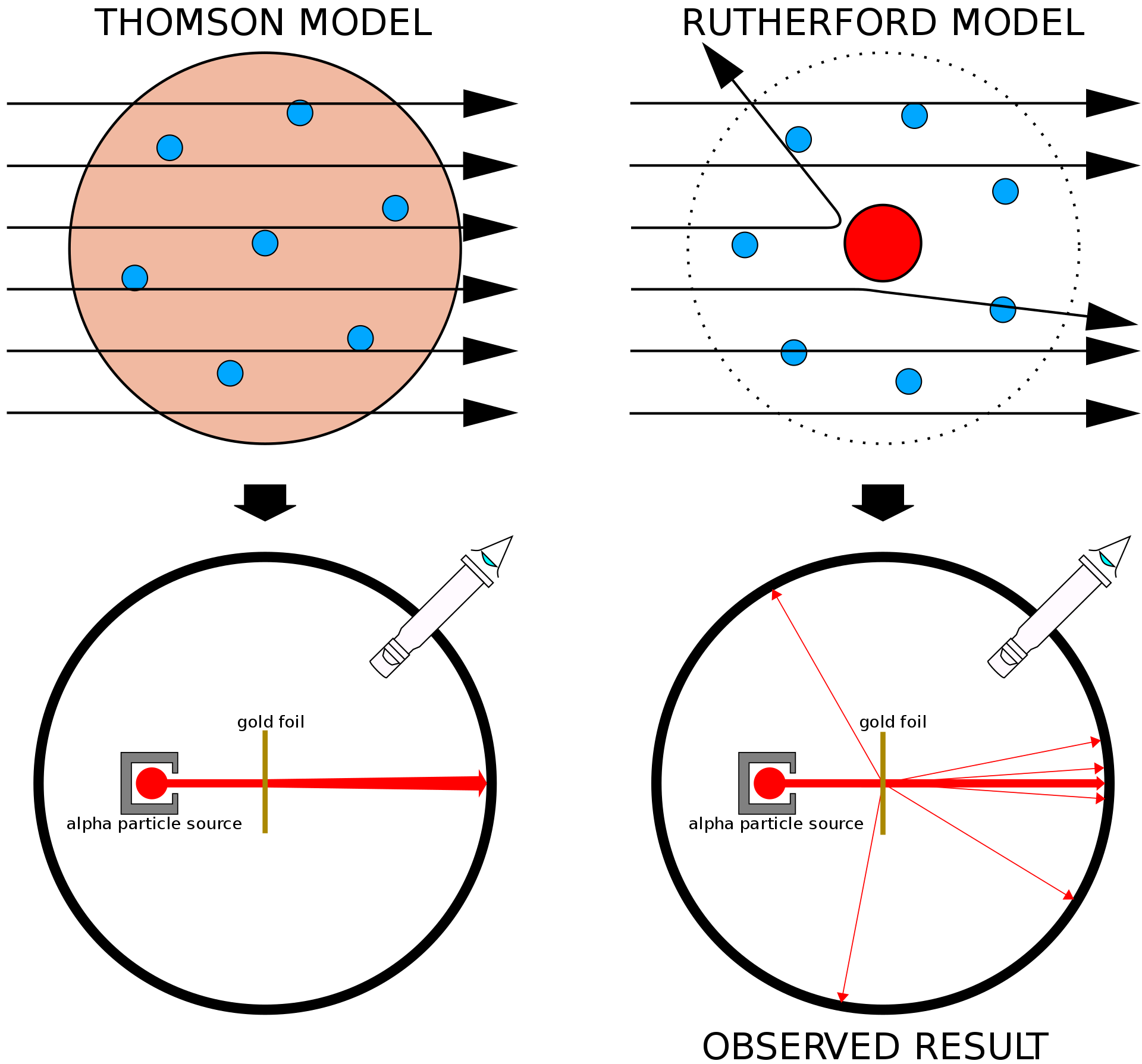
With the tools to compute scattering probability one can now look back at the seminal experiment which started nuclear physics as we now know it. The leading theory of the atom at the turn of the 20th century was Thomson’s or the plum pudding model where the electrons are held in place by a substance with positive charge that extends over the atom. In order to test this theory in 1905 Rutherford and his students Geiger and Marsden spread a few-atoms-thick Gold film and shot alpha particles (i.e. Helium, ${}^4_2$He, stripped of its electrons) at it, measuring the direction along which the particles had scattered.

The expectation from Thomson’s model is that most of the alpha particles would pass unperturbed; if they encountered an electron, which is ten thousand times lighter, they would knock it off without changing course, whereas going through the positively charge substance might have slowed them but not deflected them much. It was then to Rutherford’s reported surprise that they detected a significant number of alpha particles scattered at large angles and even backwards. They concluded that the mass of atoms must be concentrated in a small region and those backscattered particles happened to bounce of this ’nucleus’.

4.1 Rutherford cross section

With our previous knowledge we can go further than words and actually compute the scattering cross section. The interaction between the nucleus and the alpha particles is mediated by electromagnetism and we can think of the alpha particle moving in the potential generated by the Gold core so

${\mathscr{H}}_{\text{int}}(𝐱)=V_{\text{Coulomb}}={\displaystyle \frac{Z_{\text{He}}{Z}_{\text{Au}}{e}^2}{4\pi {\epsilon }_{0}r}}$ (4.1)

with $r=|𝐱|$ and ${\epsilon }_0$ the permittivity of free space.

Our matrix element for the cross section is in momentum, not space representation; to connect the two we use the favourite trick in quantum mechanics and insert the identity as

$⟨{𝐩}^{\prime }|{\mathscr{H}}_{\text{int}}|𝐩⟩={\displaystyle \int d^{3}x⟨{𝐩}^{\prime }|𝐱⟩{\mathscr{H}}_{\text{int}}(𝐱)⟨𝐱|𝐩⟩}={\displaystyle \int d^{3}x{e}^{i𝐪\cdot 𝐱}{\mathscr{H}}_{\text{int}}(𝐱)}$ (4.2)

with $𝐪=𝐩-{𝐩}^{\prime }$. That is the Fourier transform of the potential. One can perform this transform by changing to spherical coordinates:

${\displaystyle \int r^2𝑑rd(-c_{\theta })𝑑\varphi e^{i|𝐪|r{c}_{\theta }}{\mathscr{H}}_{\text{int}}(r)}={\displaystyle \frac{2\pi }{|𝐪|}}{\displaystyle \int r𝑑r\frac{e^{iqr}-e^{-iqr}}{i}\frac{Z_{\text{He}}{Z}_{\text{Au}}{e}^2}{4\pi {\epsilon }_{0}r}}$ (4.3)

The dependence on the radius $r$ is then limited to complex exponential; we know how to do this integral but how do we evaluate it given that the upper limit of integration is $r=\mathrm{\infty }$? Here the way will be to introduce an exponential factor as $\mathscr{H}\to \mathscr{H}{e}^{-r/a}$, then take $a\to \mathrm{\infty }$ which gives $e^{-r/a}(a\to \mathrm{\infty })\sim 1$. This is more justified than what you would think, after all, at a distance of about the Bohr radius of Gold we have the electron screening an even further there’s no potential. What we obtain is

$⟨{𝐩}^{\prime }|{\mathscr{H}}_{\text{int}}|𝐩⟩={\displaystyle \frac{2\pi Z_{\text{He}}{Z}_{\text{Au}}{e}^2}{4\pi {\epsilon }_0|𝐪|}}{\displaystyle \int 𝑑r\frac{e^{i|𝐪|r}-e^{-i|𝐪|r}}{i}{e}^{-r/a}}={\displaystyle \frac{Z_{\text{He}}{Z}_{\text{Au}}{e}^2}{2{\epsilon }_0}}{\displaystyle \frac{1}{{𝐪}^2+a^{-2}}}$ (4.4)

Taking our limit $a\to \mathrm{\infty }$ leaves us with ${𝐪}^2$ only in the denominator. The modulus of the transferred momentum $𝐪$ is, given that $|{𝐩}^{\prime }|=|𝐩|$:

$${𝐪}^2={(𝐩-{𝐩}^{\prime })}^2={𝐩}^2[{(1-\cos \theta )}^2+\sin {(\theta )}^2(\cos ({\varphi }^2)+\sin {(\varphi )}^2)]=4{𝐩}^2\sin {(\theta /2)}^2$$

if in addition we take the non-relativistic approximation $E_{𝐩}\simeq m$, we obtain Rutherford’s cross section:

${\left({\displaystyle \frac{d\sigma }{d\mathrm{\Omega }}}\right)}_{\mathrm{Ruth}}={\displaystyle \frac{m^2{\alpha }_{\text{em}}^2{Z}_{\text{He}}^2{Z}_{\text{Au}}^2}{4{𝐩}^4{\sin }^4(\theta /2)}}={\displaystyle \frac{{\alpha }_{\text{em}}^2{Z}_{\text{He}}^2{Z}_{\text{Au}}^2}{16E_{\text{K}}^2{\sin }^4(\theta /2)}}$ (4.5)

where $E_{\text{K}}$ is the kinetic energy, $E_{\text{K}}={𝐩}^2/2m$ and ${\alpha }_{\text{em}}=e^2/4\pi {\epsilon }_0$ is the electromagnetic fine structure constant.

4.2 Comparison with experiment

This formula gives the prediction for the scattering of a charge $Z_{\text{He}}e$ particle off a static point particle of charge $Z_{\text{Au}}e$. Integrating over solid angle (glossing over the divergence at $\theta =0$ for now) we obtain the total cross section $\sigma$, multiply this times the luminosity and you would have a prediction for the number of scatterings to compare with experimental data. We can do much better than that however. The differential cross section is a prediction for each scattering angle, if we break down our scatterings into angles we will have a function rather than a point to compare with!

Figure 2: Histogram built out of a Rutherford-like experiment with a total of 1000 scattering events.

How do we go about reconstructing such a function? In practice we cannot reconstruct a smooth function due to two main limitations and we instead obtain a distribution that looks like a coarse grained function or histogram as in fig. 2. There is a so-called systematic limitation stemming from the finite resolution in our measuring devices; we cannot measure the scattering angle with infinite precision so instead we put our particles in ‘boxes’ the size of our experimental resolution, $\mathrm{\Delta }\theta$ in this case. Then there is a statistical limitation due to the probabilistic nature of quantum mechanics and the finiteness of our dataset. In our Rutherford-like experiment we count how many particles scatter in a given range of $\theta$ but quantum mechanics gives a probability for this to happen not a deterministic prediction. Rolling a dice we have equal probability to get an even or odd number, if we roll and even number twice it doesn’t mean our probabilities were wrong. This limitation can be pushed to be smaller by measuring more and improves as $1/\sqrt{N}$, the systematic limitation however can only be overcome with better technology.

4.3 Mott cross section

This formula was derived for non-relativistic particles but is not much more work to do it for relativistic particles. Shooting particles at a Gold atom if we want to probe subatomic distances $\lambda \sim 0.1$pm we need a momenta.

$$|𝐩|=\frac{2\pi }{0.1\mathrm{pm}}=\frac{2\pi (197\mathrm{fm}\mathrm{MeV})}{100\mathrm{f}\mathrm{m}}\sim 13\mathrm{MeV}$$

where we introduced a factor $\mathrm{\hslash }$c to convert from SI to NU. While an alpha particle can achieve this momentum for $v\sim 0.003$c for an electron this momentum is well above its mass which means it is a relativistic particle (can you find its speed? $v=|𝐩|/E_{𝐩}$).

This means that the electron would be relativistic and our formula has to be corrected to Mott’s scattering cross section for no recoil

${\left({\displaystyle \frac{d\sigma }{d\mathrm{\Omega }}}\right)}_{\mathrm{Mott}}={\left({\displaystyle \frac{d\sigma }{d\mathrm{\Omega }}}\right)}_{\mathrm{Ruth}}(1-v^2{\sin }^2(\theta /2))$ (4.6)

The behaviour of this formula can be justified in the relativistic limit. It does indeed cancel for backscattering ($\theta =0$) when $v\sim 1$. This follows from conservation of angular momentum; at high energies helicity, i.e. spin along direction of motion, is a conserved quantum number. Angular momentum itself is conserved and with Coulomb’s potential there is no transfer of angular momentum. All these factors mean we can’t have a relativistic particle helicity bouncing straight back.

5 Nuclear shapes

Rutherford’s experiment taught us that the atom is mostly an electron cloud in volume and a small nucleus in its mass. One can do better than this qualitative description and put numbers in place of ‘mostly’. This chapter outlines how we do this while giving an explicit connection of wavelength and the distances we can resolve.

5.1 Form factor

A small nucleus meant in practice that we approximated it to be point-like and the potential it generated was Coulomb’s. If one has instead an extended distribution or density of charge the potential is to be found solving Laplace’s equation which gives

${\mathscr{H}}_{\text{int}}=$ ${\displaystyle \frac{Z_1{Z}_2{e}^2}{4\pi {\epsilon }_0}}{\displaystyle \int d^{3}y\frac{f(𝐲)}{|𝐱-𝐲|}}$ ${\displaystyle \int d^{3}xf(𝐱)}$ $=1$ (5.1)

where $f(y)$ is the probability density of a proton. Here we have used some of our implicit knowledge, that is that the charge $Z_{1}e$ is made up of $Z_1$ identical particles and we even gave them a name, the proton.

Propagating this change to the cross section we have the square of a more complicated Fourier transform. One can nonetheless factorize this change with a little massaging as

${\displaystyle \int d^{3}x{d}^{3}y\frac{e^{i𝐪\cdot 𝐱}f(𝐲)}{|𝐱-𝐲|}}={\displaystyle \int d^{3}z\int d^{3}y\frac{e^{i𝐪(𝐳+𝐲)}f(\text{𝐲})}{|\text{𝐳}|}}=\left[{\displaystyle \int d^{3}z\frac{e^{i\mathrm{𝐪𝐳}}}{|𝐳|}}\right]\left[{\displaystyle \int d^{3}y{e}^{i\mathrm{𝐪𝐲}}f(\text{𝐲})}\right]$ (5.2)

which allows us to write

$⟨{𝐩}^{\prime }|{\mathscr{H}}_{\text{int}}|𝐩⟩$ $={\displaystyle \frac{Z_{\text{He}}{Z}_{\text{Au}}{e}^2}{2{\epsilon }_0}}{\displaystyle \frac{F({𝐪}^2)}{{𝐪}^2}}$ $$F({𝐪}^2)=\int d^{3}y{e}^{i𝐪\cdot 𝐲}f(𝐲)$$ (5.3)

and hence a cross section

$$\frac{d\sigma }{d\mathrm{\Omega }}={|F({𝐪}^2)|}^2{\left(\frac{d\sigma }{d\mathrm{\Omega }}\right)}_{\mathrm{Ruth}}$$

This form factor depends on the scattering angle through the transferred momentum $𝐪$ so we can look at the differential distribution to find the changes wrt to Rutherford scattering but, how do we relate them to the size of the nucleus?

5.2 Energetic enough to see

Let’s start with a rough sketch of what the nucleus could be like. Consider a spherical uniform distribution which ends sharply at $r=R$. Our charge distribution is then

$f_{\mathrm{Sph}}(𝐲)$ $r$ $=|𝐲|$ (5.4)

which returns

$F({𝐪}^2)={\displaystyle \frac{3}{4\pi R^3}}{\displaystyle {\int }_0^R}{r}^2𝑑r(2\pi ){\displaystyle \frac{e^{i𝐪r}-e^{-i𝐪r}}{i𝐪r}}={\displaystyle \frac{3}{{(|𝐪|R)}^2}}\left({\displaystyle \frac{\sin |𝐪|R}{|𝐪|R}}-\cos (|𝐪|R)\right)$ (5.5)

This form factor presents a number of the features of finite size targets.

• In low energy limit $𝐪R\ll 1$ one does not have enough energy to resolve the size of the nucleus and it is effectively point-like. This can be seen taking the limit

  $$F({𝐪}^2\ll R^{-2})\to 1$$

  which you can do yourself using the expansion of sine and cosine for small argument

  $\sin (x)=$ $x-{\displaystyle \frac{x^3}{6}}+𝒪(x^5)$ $\cos (x)=$ $1-{\displaystyle \frac{x^2}{2}}+𝒪(x^4)$

  and means we will recover Rutherford’s cross section where the nucleus is described as point-like. This is evidence for our statement that to resolve distances of a size $d$ we should use particles with momentum of at least $1/d$ (in natural units).

• In the high momentum regime there will be angles $\theta$ where interference causes the cross section to approximately cancel, we can find these values as

  ${\displaystyle \frac{\sin (|{𝐪}_0|R)}{|{𝐪}_0|R}}-\cos (|{𝐪}_0|R)$ $=0$ $|{𝐪}_0|R=2|𝐩|\sin ({\theta }_0/2)R$ $\simeq 4.493,7.725,\mathrm{\dots }$ (5.6)

  If we know the momentum of the incoming particles and we can find the angle ${\theta }_0$ where our first dip would be we can determine $R$.

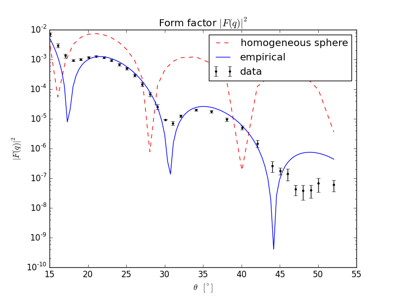
when we increase enough our projectile’s momentum a diffraction-like pattern will appear in our distribution in scattering angle. Let us look at actual data and see; fig. 2(a) contains the experimental data points in black, our naive ansatz in dashed red and a grown-up ansatz for the form factor in blue which reads

$f_{\mathrm{ph}}={\displaystyle \frac{C}{1+e^{(r-R)/a}}}$ (5.7)

with $C$ a normalization factor.

(a) Ratio of cross section to Rutherford’s cross section as a function of the scattering angle

(b) Charge distribution as inferred from scattering data

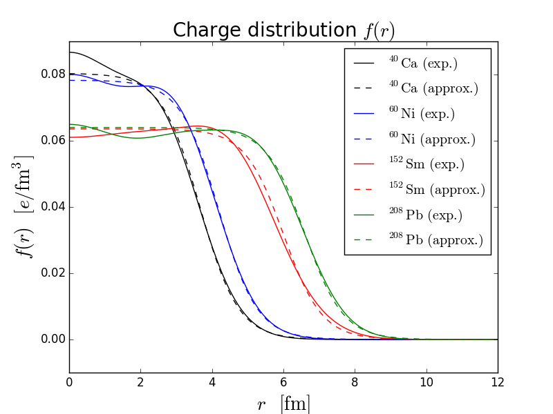
Whereas our sphere modelling does not fall squarely on top of the data it does give the ballpark value within a few degrees. In fact for enough data, we can turn it around and obtain the inverse Fourier transform of the form factor to get the charge density $f$, which is what is done in fig. 2(b).

6 Nuclear masses and binding energies

So we have seen evidence of nuclei being a few fm in radius and having integer charges compatible with a number $Z$ of copies of a Hydrogen nucleus, let’s call it proton for short, which are themselves distributed roughly homogeneously. Considering only protons however we would account for less than half of the nuclei mass. As we know now other particles of similar mass but with no electromagnetic charge make up for the missing part, neutrons, discovered by Chadwick in 1932. Ultimately the way we find out that nuclei are made up of these particles is breaking them apart, which will be discussed on the next chapter. Here we will study the force holding nucleons and protons together and the effect it has on nuclei masses.

What is the force holding nucleons together? First let’s give it a name, the strong force, we do already know some things about it:

• It is stronger than the electromagnetic force.

• It has a short range of the order of a few $\mathrm{fm}$.

• It is attractive (except for a repulsive core for distances smaller than $\simeq 1\mathrm{fm}$).

If we were to follow the successful steps of the Hydrogen atom one could think of reconstructing the force from nucleon nucleon scattering then computing the bound states from Schrodinger’s equation. This program is however faced with a number of hurdles

• The nuclear force is so strong that perturbative methods have poor convergence

• Its a many body problem with all particles of the same mass.

• Nucleons move at large speeds and the non relativistic approximation is not always valid.

Let’s have a look at the first step of this program, reconstructing the nucleon-nucleon potential as possible in principle from nucleon-nucleon scattering, we would find:

$V_{\mathrm{Ncl}}=$ $V_0(r)+V_{ss}(r)({𝐒}_1\cdot {𝐒}_2)+V_T(r)\left(3{\displaystyle \frac{({𝐒}_1𝐱)({𝐒}_2𝐱)}{r^2}}-{𝐒}_1{𝐒}_2\right)+V_{LS}(r)({𝐒}_1+{𝐒}_2)\cdot 𝐋$

$+V_{Ls}(r)({𝐒}_1\cdot 𝐋)({𝐒}_2\cdot 𝐋)+V_{ps}(r){\displaystyle \frac{({𝐒}_1\cdot 𝐩)({𝐒}_2\cdot 𝐩)}{m^2}}$ (6.1)

with ${𝐒}_{1,2}$ the spin of each nucleon and $𝐋$ angular momentum. Compare this to the Coulomb potential and you may realize why a phenomenological approach will be adopted here.

Rather than solving for the bounds states of a multi-particle system with a complicated potential we can just ask Nature directly what the binding energies are. This turns out to be a very straightforward experimental determination, the reason behind given by Einstein’s mass formula.

6.1 Binding energy

The masses of the proton and neutron, our nuclei building blocks are:

$M_p=938.27\text{MeV}=1.0073\text{u},M_n=939.57\text{MeV}=1.0087\text{u}$ (6.2)

where $u$ is the atomic mass unit defined by the nuclear mass of Carbon $M({}_6^{12}$C$)=12u$. The most common form of Helium is made up of two protons and two neutrons which we denote ${}_2{}^4\text{He}$ with superindex total number of nucleons (mass number) and subindex number of protons (atomic number). So one would expect the mass of Helium to be

$M$ $=2M_p+2M_n=2\times 1.0073\text{u}+2\times 1.0087\text{u}$

$=4.032\text{u}$ (6.3)

So what’s the mass of the He nucleus? Nature tells us is

$M{(}_2^4\text{He})=4.0015\text{u}.$ (6.4)

Comparing these two values of mass reveals one of the most striking results in nuclear physics. The mass of the nucleus is less than the mass of its constituent parts; what is this deficit? Binding energy $B$, the connection energy-mass given by Einstein’s mass relation $m=E/$c${}^2$. For Helium we have

$B(4,2)={\displaystyle \frac{E_B}{c^2}}=2M_p+2M_n-M{(}_2^4\text{He})=0.031\text{u}.$ (6.5)

To dismantle a nucleus we have to put in this amount of energy as shown in fig. 3. This energy corresponds to the mass difference between free and bound nucleons and is therefore also called the mass defect.

Figure 3: In order to break the bond of a nucleus into separate nucleons energy is required (e.g. by an energetic photon).

The mass defect is clearly manifest in nuclear physics, but it does not mean that it only happens here. In atomic physics electrons are also in bound states and this will give a mass defect only here binding energies of $13$eV are 8 orders of magnitude smaller than atomic masses and it is safe to neglect it.

The exercise can be repeated for all elements of the periodic table giving us a wealth of data about the nuclear force. To classify our nuclei we use two numbers, as

Atomic number:

the number of protons in the nucleus. Because the number of proton is the same as the number of electrons in a neutral atom the atomic number specifies the chemical properties of the atom. It is normally denoted with $Z$

Mass number:

the number of proton and neutrons. As its name suggests it is roughly related to the mass of the nucleus in atomic mass units. It is usually denoted with $A$.

A nucleus with atomic number $Z$ and mass number $A$ has therefore $N=A-Z$ neutrons. Nuclides are represented as ${}^{A}X$, ${}_Z{}^{A}X$ or ${}_Z{}^{A}X_N$ with $X$ the chemical symbol for the atom.

The binding energy $B(A,Z)$ of a nucleus with atomic number $Z$ and mass number $A$ is the difference between its atomic mass and the sum of the mass of its constituents.

$B(A,Z)=ZM({}^1\text{H})+(A-Z)M(n)-M(A,Z)$ (6.6)

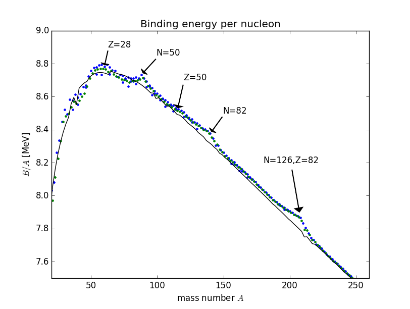
Here, $M({}^1\text{H})=M_p+m_e$ includes the masses of the proton and of the electron. This formula assumes that the energy difference coming from the electron binding energies is negligible (it is $\approx 13.6\mathrm{eV}$). The binding energies for all nuclei are shown in Fig. 3(b).

(a) Radius of different nuclei as a function of cubic root of the mass number.

(b) Binding energy per nucleon as a function of the mass number for the most stable isobar (same $A$) together with the prediction of the semi-empirical mass formula (eq. 6.2) for odd $A$ nuclei (black line).

Figure 4: Radius and binding energy per nucleon.

6.2 The liquid drop model

The binding energies cannot be predicted accurately from first principles for the reasons outlined in the beginning of this chapter. Instead an approximate formula can be postulated based on physical arguments, with parameters to be determined experimentally, the so-called Bethe-Weizsäcker or semi-empirical mass formula based partially on the liquid drop model

$B(A,Z)$ $=E_{\text{Volume}}-E_{\text{Surface}}-E_{\text{Coulomb}}-E_{\text{Asymmetry}}\pm E_{\text{Pairing}}$

$=a_{V}A-a_s{A}^{2/3}-a_c{\displaystyle \frac{Z^2}{A^{1/3}}}-a_a{\displaystyle \frac{{(N-Z)}^2}{4A}}+{\displaystyle \frac{\delta }{A^{1/2}}}$ (6.7)

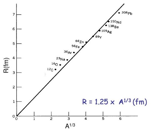
Some of these terms are motivated by a comparison between the nucleus and a liquid drop. Both the nucleus and a drop of liquid contain large numbers of particles, are homogeneous and incompressible and their mass density drops off sharply at the boundary. In this picture, the binding energy of the nucleus corresponds to the vaporisation heat of a liquid. The radius of the nucleus, given the approximately constant density, is taken proportional to $A^{1/3}$ (you can see how good of an assumption this is on fig 3(a)).

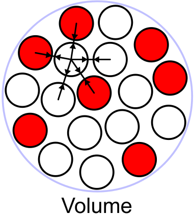
Volume term

[$E_{\text{Volume}}=a_{V}A$] The strong force between nucleons is short-range, unlike the Coulomb force or gravity. Just like molecules in a liquid, nucleons only interact with other nucleons that are close enough, so the contribution to the potential energy scales with the mass number $A$. This can be understood as follows, the attractive nature of the force means its energetically favourable for a nucleon to surround itself with other nucleons, but it can only be surrounded by a few and the ones one layer away do not sizably contribute to binding energy. This means there is a constant binding energy per nucleon and the total binding energy $B$ scales with A. Since the volume of a sphere is given by $4/3\pi R^3\propto A$, this term is called the volume term.

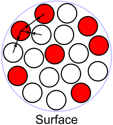
Surface term

[$E_{\text{Surface}}=a_s{A}^{2/3}$] In the above description we neglected the fact that the density of neighbours is smaller for nucleons at the boundary of the nucleus, these will not contribute as much as those in the middle of the nucleus. This term corrects for this effect and is proportional to the area of the nucleus and since the area scales as $\text{area}=4\pi R^2$, we have a term proportional to $R^2={(A^{1/3})}^2=A^{2/3}$. The equivalent in a liquid drop is the surface tension. Both the liquid drop and the nucleus are spherical, because this shape combines the largest volume with the smallest surface.

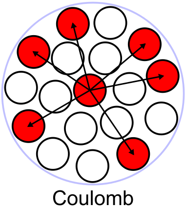
Coulomb term

[$E_{\text{Coulomb}}=a_c{Z}^2/A^{1/3}$] Electromagnetic interactions push the nucleus apart. This has no analogy in a liquid drop. The potential for each proton is proportional to the number of other protons so it will be proportional to $Z(Z-1)$. The Coulomb potential is proportional to $V(r)=\alpha /r$ so we expect a dependence proportional to $1/R=A^{-1/3}$, for large values of $Z$ we can replace $Z(Z-1)$ with $Z^2$.

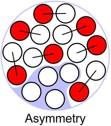
Asymmetry term

[$E_{\text{Asymmetry}}=a_a{(N-Z)}^2/(4A)$] This term is a quantum effect and can also not be explained in analogy with the liquid drop. Since both neutrons and protons are fermions (which carry spin $1/2$ ) Fermi statistics enforces that no two identical nucleons can be in the same state. To illustrate how this term arises we can imagine that the neutrons and protons have the same energy levels, and they fill the lowest $n$ levels if there are $n$ nucleons of one type. If we start from a nucleus with equal number $n$ of protons and neutrons both type will have their $n$ lowest energy state filled. If we now try to replace a neutron with a proton, this cannot work straight-forwardly because the corresponding energy level is already occupied by a proton, so this new proton will have to go into a higher energy level, hence reducing the binding energy. Nuclei with a symmetric number of neutrons and protons can be packed tighter. This term measures the difference between the number of neutrons and protons and is therefore proportional to $A-2Z=N-Z$.

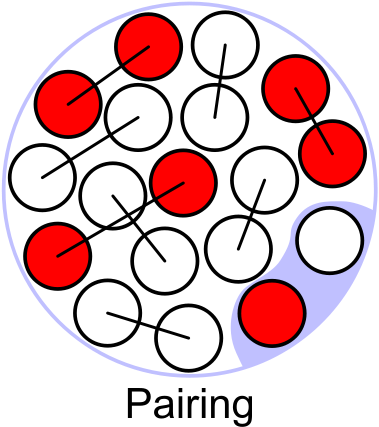
Pairing term

[$E_{\text{Pairing}}=\delta /A^{1/2}$] Nuclei with even numbers of protons and neutrons are more stable. The reason is again a quantum effect and can not be explained by analogy with the liquid drop. In terms of shells, it can be explained by the fact that two different nucleons with opposite spin can be on the same shell, whereas a third nucleon would need to be on the next shell, i.e. lead to a bigger, more weakly bound nucleus. So we expect different values of $\delta$ for both protons and neutrons appearing in even numbers, one even and one odd and for both in odd numbers. The scaling as a function of $A$ is found to be as $A^{-1/2}$.

(6.8)

Although this model of the binding energies of nucleons is descriptive and we can only motivate the terms with qualitative explanations it does a good job of describing nature with a relatively small number of inputs as you can see in fig 3(b).

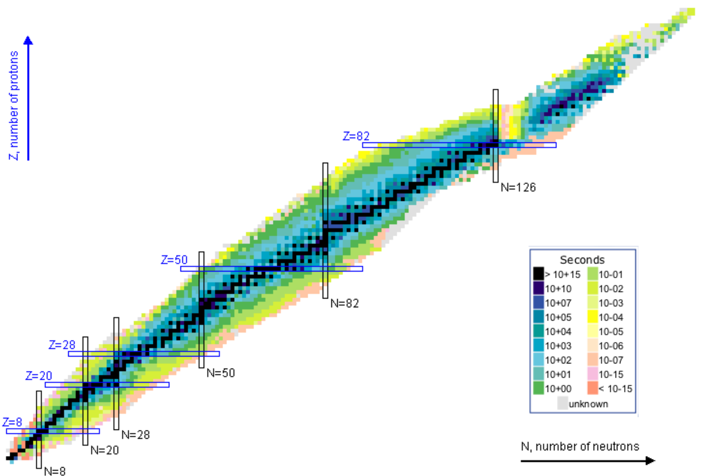
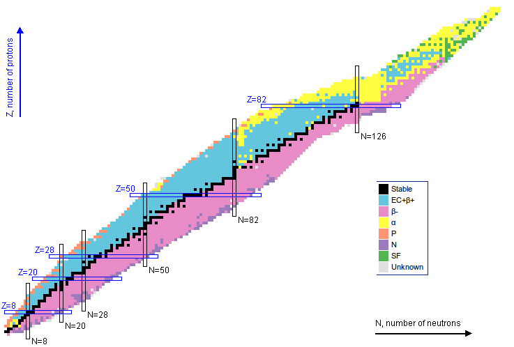
7 Nuclear stability

Not all bound states of protons and neutrons result in a stable nucleus. There are a relatively small number of nuclides that can be observed, with a smaller that are stable. The stable nuclides are shown in Fig. 5. The mass formula can tell us if a given transition is energetically viable, that is explicitly decays can occur if the difference of masses of initial state and final state, here called $Q$, is positive

$Q=\text{parent mass}-\text{daughter masses}>0.$ (7.1)

This does not tell us however how it happens or if it happens at all. There are a first a few rules that decays should satisfy as we have found through experiments

• Conservation of baryon number

• Conservation of lepton number

• Conservation of angular momenta

• For strong and electromagnetic decays, conservation of parity

Figure 5: Stability of the nuclides as a function of the number of protons $Z$and the number of neutrons $N$. The color coding indicates the lifetime in seconds. Figure taken from [3].

Neutrons and protons are assigned a baryon number of one and this conservation means that their total number will not change. Equivalently electron $e^{-}$ and electron neutrino ${\nu }_e$ have electron number 1 but their anti-particles the positron $e^{+}$ and anti-neutrino ${\overline{\nu }}_e$ electron number $-1$.

Nuclei have a baffling range of lifetimes from ms to millions of years. This reflects both the fact that there are different mechanisms for decay and that these mechanisms are very sensitive to differences in bound states.

Figure 6: Fraction of atoms remaining as a function of time.

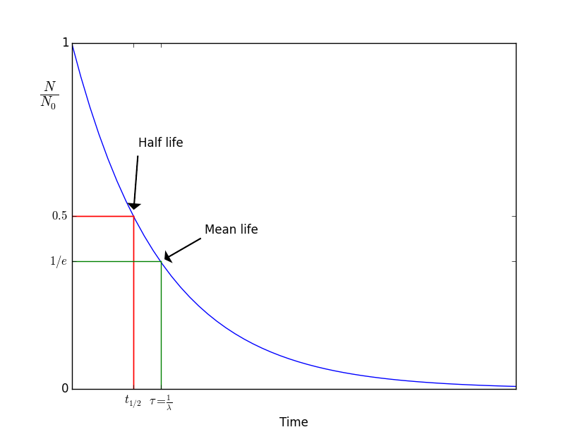
We characterize how long does a nucleus live by $\lambda$, its decay rate. If we have a number of unstable states $N$ we find that the number of decays per unit time proportional to the number of states

${\displaystyle \frac{dN}{dt}}=-\lambda N,\Rightarrow \mathit{\hspace{1em}}N(t)=N_0{e}^{-\lambda t}.$ (7.2)

With $\lambda$ the proportionality constant. The solution of this equation tracks the number of states $N$ after a time $t$ has elapsed. We can ask questions then like how long does it take until only have of the atoms are left? The answer to this is is called the halflife of a sample,

$N(t_{1/2})$ $={\displaystyle \frac{N_0}{2}}=N_0{e}^{-\lambda t_{1/2}}$

$\Rightarrow t_{1/2}={\displaystyle \frac{\ln (2)}{\lambda }}.$ (7.3)

We can ask a slightly different question: how long does it take on average for a nucleus in the sample to decay? In this case the answer is given by the mean lifetime,

$dP$ $={\displaystyle \frac{-dN}{N_0}}=-{\displaystyle \frac{1}{N_0}}{\displaystyle \frac{dN}{dt}}dt=\lambda e^{-\lambda t}$ (7.4)

$\tau \equiv ⟨t⟩$ $={\displaystyle \int t𝑑P}={\displaystyle \frac{1}{N_0}}{\displaystyle {\int }_0^{\mathrm{\infty }}}\lambda tN(t)𝑑t={\displaystyle \frac{1}{\lambda }}{\displaystyle {\int }_0^{\mathrm{\infty }}}𝑑xx{e}^{-x}={\lambda }^{-1}$ (7.5)

The mean lifetime is related to the halflife by $t_{1/2}=\tau \ln (2)$. Figure 6 shows the exponential decay of the number of nuclei and the lifetime and half time.

The frequency of decays in a material is called the activity

$$A=-\frac{dN}{dt}=\lambda N$$

Commonly used units for the activity are Becquerel ($1\mathrm{B}\mathrm{q}=1\text{decay}/\mathrm{s}$) or Curie ($1\mathrm{C}\mathrm{i}=3.7\cdot {10}^{10}\mathrm{Bq}$). The activity of a sample decreases with time as the number of candidate nuclei for a decay diminishes,

$A(t)=\lambda N(t)=\lambda N_0{e}^{-\lambda t}$ (7.6)

The range of lifetimes for nuclei spans many orders of magnitude: some nuclides live for a mere fs after being produced in the lab while others have a lifetime longer than thousands of years and are present on earth contributing to the environmental radiation. The SI unit for measuring the radiation dose is the sievert, Sv, and is determined by energy absorbed by kilogram of tissue times a quality factor $\overline{\gamma }$ which depends on the type of radiation $(\beta ,\gamma ,\overline{\gamma }=1;\alpha ,\overline{\gamma }=20)$. Typical doses we are exposed to are in the mSv per year.

8 Beta-decays (decays with constant A)

These are decays mediated by the weak interactions, which stem from a third type of force different from the strong or electromagnetic. The basic interaction mediates the process of neutron decay; a free neutron has a lifetime of about $\tau =879.6\mathrm{s}=14$min 40 s and decays into a proton, an electron and a neutrino through the weak interaction

$$n\to p+e^{-}+{\overline{\nu }}_e$$ (8.1)

this process is called $\beta$ decay and it explains why there are no free neutrons even though there are free protons. Neutrons can be long lived when they are part of a nucleus, energetically neutron decay as above releases $Q=0.8$MeV but average binding energy per nucleon are 10 times that, see 3(b). In fact the opposite effect can also happen if the nucleus resulting from a proton changing into a neutron is less massive. This can be triggered by a reduction in the Coulomb energy and depending on the neutron-proton imbalance may result in the newly created neutron taking a lower energy state than the proton. Nuclei with large number of protons will tend to exchange protons for neutrons and nuclei with large numbers of neutrons compared to protons will tend to exchange protons for neutrons. This processes called $\beta$-decay do not change the mass number $A$ but change $Z$.

Three processes are possible, all using variations of the $\beta$-decay formula (8.1) by moving particles between final and initial state. All of them include neutrinos whose mass can be neglected.

${\beta }^{-}$ decay:

A neutron in the nucleus decays into a proton, an electron and an electron anti-neutrino.

$n\to p+e^{-}+{\overline{\nu }}_e$ (8.2)

This decay within a nucleus reads,

${}_Z{}^{A}X_N{⟶}_{Z+1}^A{Y}_{N-1}+e^{-}+{\overline{\nu }}_e.$ (8.3)

Such a decay is possible if the mass difference between the parent and daughter nuclei is large enough to “afford” the creation of the electron an neutrino. In terms of atom masses the condition is :

$M(A,Z)>M(A,Z+1)$ (8.4)

where the fact that we use atom masses takes the additional electron produced in the decay into account since the daughter nucleus has one more electron than the parent.

${\beta }^{+}$ decay:

A proton in the nucleus is changed into a neutron by emitting a positron and a neutrino:

$p\to n+e^{+}+{\nu }_e$ (8.5)

Inside a nucleus this reads

${}_Z{}^{A}X_N{⟶}_{Z-1}^A{Y}_{N+1}+e^{+}+{\nu }_e.$ (8.6)

For this process to happen the mass difference between the nuclei should be large enough to ”buy” the mass of the positron. In terms of atomic masses the condition is

$M(A,Z)>M(A,Z-1)+2m_e$ (8.7)

we need to add twice the mass of the electron on the right-hand side to account for the mass of $Z$ electrons and 1 positron.

electron capture:

in this case we consider the case in which an electron from the atom combines with a proton to give a neutron and a neutrino:

$p+e^{-}\to n+{\nu }_e,$ (8.8)

so that for this reaction inside the nucleus

${}_Z{}^{A}X_N+e^{-}{⟶}_{Z-1}^A{Y}_{N+1}+{\nu }_e,$ (8.9)

and for this process to occur the condition is less stringent because no energy is needed to produce a positron or electron, only the (negligible) energy for the neutrino is needed. The condition is

$M(A,Z)>M(A,Z-1)+ϵ$ (8.10)

where $ϵ$ is the energy of the excited state of the nuclide ${}_{Z-1}{}^{A}Y$ produced. For this process to happen there needs to be some overlap between the electron wave function and the nucleus. This is more likely to be the case for $s$-shell electron since there the radial wave function has a non-zero value at the origin. Also the higher the charge of the nucleus the closer the electron wave function is concentrated close to the nucleus, so electron capture gets more likely for larger nuclei. Electron capture is always possible when ${\beta }^{+}$-decay is allowed but the reverse is not true: if the mass difference between two isobars is smaller than $2m_e$ only electron capture is possible.

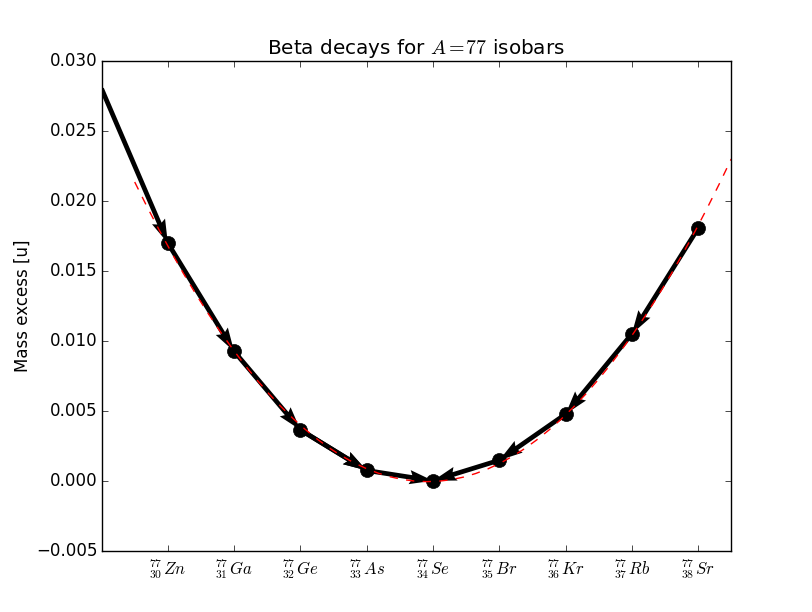
Since these decays do not change $A$ we can quantify this by looking at the semi-empirical formula eq. 6.2 and eq. (6.6) for a fixed value of $A$, and substituting $N=A-Z$

$M(A,Z)=(A-Z)M_n+Z(M_p+m_e)-a_{V}A+a_s{A}^{2/3}+a_c{\displaystyle \frac{Z^2}{A^{1/3}}}+a_a{\displaystyle \frac{{(A-2Z)}^2}{4A}}-{\displaystyle \frac{\delta }{A^{1/2}}},$ (8.11)

we find that the mass formula is quadratic in $Z$ so we expect the masses of the isobars to fit on a parabola.

In the case of odd $A$ we have one parabola, as shown in Figure 7. In such a case only one isobar is the lowest and is $\beta$-stable. All other isobars can decay to that stable isobar.

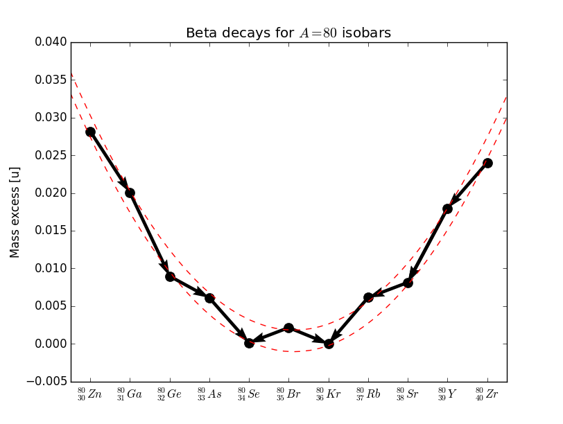
In the case of even $A$ nuclei there are two parabolas because of the pairing term. An example is shown in Figure 7. In some cases we are in a situation where there are two nuclides of the even-even type lower than a nuclide of odd-odd type.

Figure 7: Mass differences between isobars and the lightest isobar for $A=77$ (left) and $A=80$ (right). The arrows represent $\beta$-decays.

9 A-changing decays

Weak or $\beta$ decays change the charge of a nucleon but leave the nucleus with the same number of nucleons $A$. Electromagnetism and the strong force cannot do this since they preserve both the number of protons and neutrons but they can mediate the rearranging of these into separate daughter nuclei. This occurs mostly in 3 processes

i) Proton and neutron emission

Very proton or neutron rich nuclei are so unstable that they emit a single proton or neutron before it can undergo a beta decay. This is a very rare process that only occurs in a small number of nuclei. The decay formula for these processes are

Neutron emission: ${}_Z{}^{A}X_N{⟶}_Z^{A-1}{Y}_{N-1}{+}_0^1{n}_1,$ (9.1)

Proton emission: ${}_Z{}^{A}X_N{⟶}_{Z-1}^{A-1}{Y}_N{+}_0^1{p}_0.$ (9.2)

and they take place if

Neutron emission: $M(A,Z)>M(A-1,Z)+M_n$ (9.3)

Proton emission: $M(A,Z)>M(A-1,Z-1)+M({}^{1}H).$ (9.4)

Figure 8: Left panel: Potential of an $\alpha$-particle as a function of the distance to the nucleus. Right panel: Potential for the two daughters in a fission process as a function of the separation.

ii) $\alpha$-decay

Another possibility for decay is the $\alpha$-decay where an ${}^{4}He$ nucleus, also called $\alpha$-particle is emitted. This decay reduces $Z$ by two units and $A$ by four,

${}_Z{}^{A}X_N{⟶}_{Z-2}^{A-4}{Y}_{N-2}+{}_2{}^4\text{He}_2.$ (9.5)

It occurs often for heavy nuclei for which binding energy per nucleon is smaller the larger the mass number, as show in fig. 3(b). For this decay to happen the mass of the atom must satisfy:

$M(A,Z)>M(A-4,Z-2)+M(4,2)$ (9.6)

We can estimate the probability for this decay by considering the effective potential that the $\alpha$-particle is subject to, sketched on the left-hand side of fig 8. Outside of the nucleus (that is further than the range of the nuclear force) the alpha particle only feels the Coulomb potential of the remaining $Z-2$ protons in the nucleus whereas inside the nucleus the attractive strong force is simplified to produce a square-well potential. For positive total energy then there is a chance that the $\alpha$ particle tunnels out of the well.

To estimate the likelihood of the $\alpha$ particle escaping we can first consider the simplified case of a particle directed towards a thin wall as in fig. 9. The time-independent Schrodinger equation reads

$\left(-{\displaystyle \frac{1}{2m}}{\displaystyle \frac{{\partial }^2}{{\partial }^{2}x}}+V(x)\right)\mathrm{\Psi }$ $=E\mathrm{\Psi }$ $V(x)$ (9.7)

The solution gives us the wave-function regions (I) and (II) as

${\mathrm{\Psi }}_{\mathrm{I},\mathrm{II}}$ $=e^{ix{p}_{(\mathrm{I}),(\mathrm{II})}}$ (9.8)

Figure 9: The wave-function of a particle in the potential of eq. (9.7)

The probability that the particle tunnels out through our thin wall is then proportional to the square of the wave-function amplitude at $x=\mathrm{\Delta }x$, that is Exp$(-\sqrt{2m(V_{\mathrm{II}}-E)}\mathrm{\Delta }x)$. This result can be applied to any potential if we break it down into thin slices to give an expression:

$\mathrm{\Psi }(x)=\mathrm{Exp}\left(-{\displaystyle {\int }_0^x}𝑑x\sqrt{2m(E-V(x))}\right)\equiv e^{-G}$ (9.9)

where $G$ is the Gamow factor. With our approximation to the potential we have $x\to r$ and $V(r)\sim 1/r$ whereas the limits of integration are given by the size of the nucleus $R$ and the energy $E$ which sets the ‘exit’ radius $r_o$ as $V(r_o)=E$. The probability of decay will scale with the square of this exponential which means that changes in Gamow factor will be greatly amplified in the resulting lifetime. This effects accounts for the wider range of lifetimes for nuclei that decays via $\alpha$ decay.

iii) Nuclear fission

$\alpha$-decay is only one case in which the nucleus splits into several smaller nuclei. If we look at the energy as we pull the two parts of a nucleus apart we can reconstruct the potential as a function of the distance between the two parts which is sketched in fig. 8. Starting from the ground state of the parent nucleus (which we assume to be spherically symmetric) at first the surface energy dominates and we have to input energy to stretch it out, but at some finite distance this is overcome by the electromagnetic interaction whose force tries to push the two same-charge daughter nuclei apart.

Figure 10: Decay modes in the $N$-$Z$ plane. Data from [3]

The height of the barrier is called the activation energy. Very few nuclides decay through spontaneous fission, in most cases $\alpha$-decay is more likely (see fig. 10). The probability of fission increases with $Z$ and is more likely for heavy nuclides. Fission processes can be induced by exposing the nuclides to a flux of neutrons. If an atom absorbs a neutron it will acquire its kinetic energy (although part of it will be needed to produce the daughter nucleus recoil) and it also gains the bounding energy associated with the additional neutron. This additional energy can bring the nucleus energy above the fission barrier, triggering the fission of the nucleus.

10 Nuclear power

Energy is produced in each nuclear decay and can be a priori extracted for our use. Radioactive substances will however follow the exponential decay law and disappear within a period of a few lifetimes which is a problem for storage. Instead if one can find a stable substance which combined or sparked by another undergoes a reaction and produces energy we have a viable energy source. The qualitative process is like combustion with the quantitative difference being that where chemical bounds rearrange to produce an energy of around eV per reaction; nuclear energy is a million times more efficient. Here we will outline how this energy is harnessed in fission reactors and a brief sketch of how this might be possible in fusion in the future.

Fission

As we pointed out a neutron can be absorbed by a nuclei and trigger fission, in the case of ${}^{235}U$,

$\mathrm{fission}$ ${}_0{}^{1}n+{}_{92}{}^{235}U\to {}_{92}{}^{236}U⟶{}_{56}{}^{141}\mathrm{Ba}+{}_{36}{}^{92}\text{K}r+3_0^{1}n$ (10.1)

where we observe that there are three neutrons produced in the reaction; if they were to go on to excite other ${}^{235}$U nuclei past their activation energy we would have ourselves 9 neutrons and the making of a chain reaction. This feature helps sustain fission but it also requires monitoring and counterbalance.

Figure 11: Cross sections for induced fission and radiative capture for the two main isotopes or uranium. The shaded regions represent the typical energies for thermal neutrons (around 0.025 eV) and neutrons from the fission process (around 1 MeV). Data from [4]

The balance is provided in part by Uranium itself, in practice the produced neutrons do not always produce fission when absorbed, one can also have photon emission as the outcome

$\mathrm{rad}.\mathrm{caputure}$ ${}_0{}^{1}n+{}_{92}{}^{235}U\to {}_{92}{}^{236}U⟶{}_{92}{}^{236}U+\gamma$ (10.2)

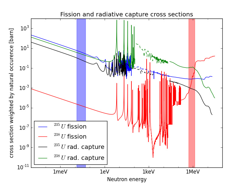
In addition ${}^{235}$U is not found in Nature in isolation but it occurs with a split of 99% ${}^{238}$U and 0.7% ${}^{235}$U. Figure 11 shows the cross section for the absorption of a neutron by these two isotopes of uranium; here we can see that for ${}^{238}$U radiative capture dominates for most of the range.

$\mathrm{rad}.\mathrm{caputure}$ ${}_0{}^{1}n+{}_{92}{}^{238}U\to {}_{92}{}^{239}U⟶{}_{92}{}^{239}U+\gamma$ (10.3)

In particular it does so for MeV neutrons which are produced in fission (with a peak slightly lower than $1\mathrm{MeV}$) which is the reason why uranium in the earth crust does not undergo a fission chain reaction. In fission power plants reaction is kept going under control with the combination of three ingredients

• Fuel Uranium with an isotope composition close to its natural abundance. One can read from fig. 11 what is more likely to occur to a neutron from fission given its energy by identifying the largest cross section.

• Moderator For these neutrons to be mainly recycled into another fission process they are cooled down by the moderator. This substance, rich in neutrons but light enough to sizably bounce off an scattering with a neutron, is commonly heavy water or graphite.

• Control rods In order to decrease the rate of the reaction, control rods of a material that absorbs neutrons can be inserted in the fissible material, with common materials being Boron.

An sketch of a fission reactor is shown in fig. 12.

Figure 12: Left: Schematic representation of the moderator and fuel arrangement in a nuclear reactor. Right: Breazeale Nuclear Reactor at the University of Pennsylvania.

Fusion

A drawback of fission is the production of radioactive materials with a thousand year lifetime whose radiation is armful. While safe disposal of this products should solve the problem, there is the (so far unrealized) possibility of using nuclear reactions which do not produce toxic materials.

Fusion makes use of the tightly bounded ${}^4_2$He nucleus to output energy. The reaction considered is

$${}_1{}^3\mathrm{H}+{}_1{}^2\mathrm{H}⟶{}_2{}^4\text{He}+n$$

which releases some $17.6$MeV.

One of the challenges of using this reaction for outputing energy is that first the tritium and deuterium must be heated enough to be able to overcome the electromagnetic repulsion between them to KeV (temperatures). At these temperatures they are stripped of electons and the fuel is therefore a charged very hot substance, a plasma which is handled by magnetic fields in smart configurations. For these and other reasons fusion presents a challenge which we haven’t met yet even if there’s progress in experiments like ITER in France.

11 Shell model

The wealth of data on nuclear masses allowed us to learn about the strong interaction and model the binding energies it produces with some success in terms of the phenomenological drop formula. This description however cannot explain some outstanding features in the data nor it does tell us about excited states. Indeed one of the signals of a state being composite (other than the obvious “it can be broken apart”) is that it has excited states that correspond to less tightly bounded combinations of its constituents.

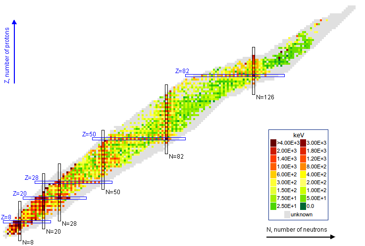
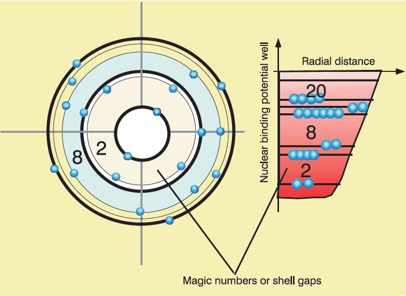
Looking at the data we find that certain nuclei with so-called magic numbers both require a large amount of energy to transition to their first excited state and have larger binding energies per nucleon than its neighbours see figs 13, 3(b). The nuclear shell model provides an explanation.

We have seen that the nucleon potential is more complex than the Coulomb potential that describes the atom; this nonetheless does not prevents us from employing some of the techniques of atomic physics, it just means they will have a smaller range of applicability and less precision on its prediction. For a simple case where we can expect some success consider a nucleon in the effective potential induced by the rest of the nucleons. We assume that this potential is spherically symmetric and that the remaining $A-1$ nucleons combine to have 0 total angular momentum (this is usually the case if $A-1$ is even). The solution to Schrodinger’s equation will then be labelled by a principal quantum number $n$ for the radial solutions and an angular momentum index $L$ for the spherical harmonic function $Y_{L,m}(\theta ,\varphi )$ and a total angular momentum index $J$, which in our case given neutron and protons have $S=1/2$ is $L\pm 1/2$. Spin-statistics tells us that no two fermions can be on the same state so we expect the protons to settle on the lowest energy unfilled states and the same for neutrons but since they are distinct fermions they fill their own set of states. We will use spectroscopic nomenclature as $n{L}_J$ with $L=s,p,d,f\mathrm{\dots }$.

If we ignore the nuclear spin in a first stage, the situation is that of the Hydrogen atom, only now our potential is short range ($\sim$ fm) which means we can approximate it to roughly follow the nucleon density that we derived from experiment in chapter 5

Figure 13: First excited state energy. The highest energies (and hence the most stable states) are concentrated around proton and neutron numbers equal to 2,8,20,28,50,82,126

Figure 14: Illustration of the shell model, the potential and magic numbers.

Figure 15: Energy levels in a harmonic oscillator (H.O.), and infinite potential well (ISQ), in the Saxon-Woods potential before (WS) and after including the spin-orbit coupling (WS+SO). Figure taken form [2]

$V(r)=-{\displaystyle \frac{V_0}{1+e^{(r-r_0)/a}}}$ (11.1)

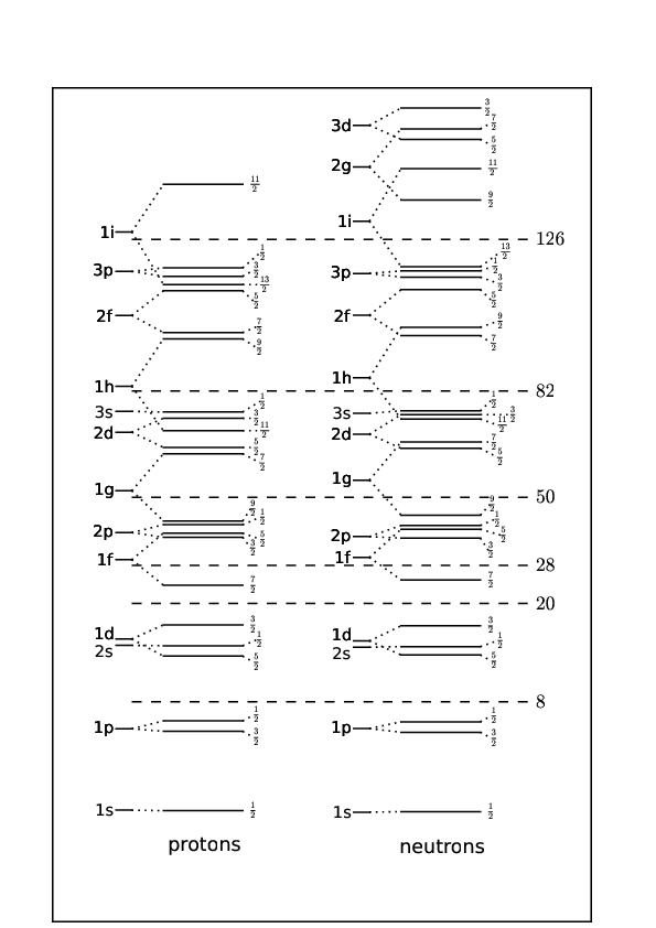
with parameters $r_0$ and $a$ fitted from data and this being called the Saxon-Woods potential (WS). With this potential we obtain the levels shown in the central part of Figure 15, (WS) for comparison shown together with the energy states of a harmonic oscillator (H.O.) and infinite square well (ISQ). This does account for why ${}^4_2$He is so tightly bound: two neutrons and two protons fill the first shell and there is a considerable gap till the next energy state. For higher $A$ neglecting the spin is not a good approximation, but given our simplified scenario with the rest of nucleons having no net angular momentum, there is only one other term to consider in our potential, spin orbit coupling:

$$V_{\text{LS}}=V_{LS}(r)𝐋\cdot 𝐒$$

Whose correction to the energy can be estimated, first computing the average of the spin coupling as we do in atomic physics:

$J(J+1)$

(11.2)

Since $S=1/2$ total angular momentum $J$ can take two values for given L: $L+1/2$ or $L-1/2$ and the energy split:

$\mathrm{\Delta }{E}_{SO,nL}$

(11.3)

We find experimentally that the coefficient is negative so that unlike for the electron levels in the hydrogen the energy level with the higher value of $J$ is the lower lying one. The result of including this contribution is shown on the right of Figure 15 and results in splits between levels consistent with the magic numbers. In practice the proton and neutron potentials can have slightly different shapes resulting in small differences in the ordering of the shells within a band, but not affecting the magic numbers, see Figure 16.

Figure 16: Energy levels for protons and neutrons. The ordering within a band are different for higher levels, but the structure in bands with magic number of nucleons is the same.

11.1 Spin and parity of nuclei

The parity of a state is given by its eigenvalue under the operation $𝐏:$ $𝐱\to -𝐱$

$$𝐏\mathrm{\Psi }=\pm \mathrm{\Psi }$$

In particular for orbital angular momentum we can deduce the parity by the spherical harmonic property

$$𝐏Y_{L,m}(\theta ,\varphi )=Y_{L,m}(\pi -\theta ,\varphi +\pi )\to {(-1)}^L{Y}_{L,m}(\theta ,\varphi )$$

Composite states have parity equal to the product of their individual parities. Electromagnetism and the strong interactions conserve parity which means it is a useful quantum number to label our states and derive selection rules.

In addition to explaining the location of magic quantum numbers, the shell model can predict parity and total angular momentum for ground states in certain cases.

Even-even

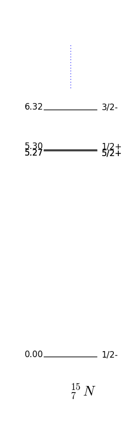
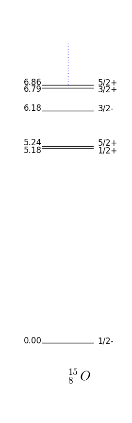
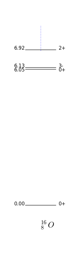
If we have an even number of protons and neutrons we can expect the parity to be +1 since for every nucleon we can find another with the same parity. As for angular momentum we expect nucleons to pair up and give no net total as in the Hydrogen atom. These approximations are specially good for magic numbers with full shells. The prediction is then $J^P=0^{+}$ as we can verify in fig. 17 for the doubly magic ${}^{16}_8$O

Even Odd

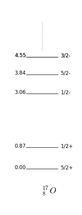
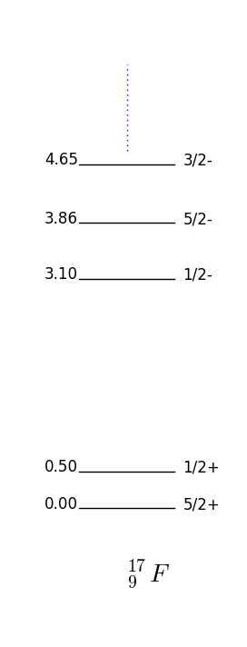
In this case the parity and momentum will be given by the unpaired nucleon, that is, $J^P={(L\pm 1/2)}^L$. This is again a very good approximation for the unpaired nucleon being one more than or one short of (also called hole) a magic number. For example ${}^{17}_9$F has one extra proton on top of a closed shell and by fig. 16 one has $J^P=5/2^{+}$ which is what is observed fig. 17.

Odd-odd

Here the total parity and angular momentum is the combination of the unpaired proton and neutron, but among the different possibilities the shell model does not tell us which to choose.

Figure 17: Energy levels for nuclei with proton and neutron numbers close to the magical number 8.

11.2 Excited states

Filling in the lowest energy states with our protons and nucleons the shell model can predict some of the nuclei ground state properties. If we consider now one or more of our nucleons not in the lowest energy state we can study excited states.

Figure 17 shows the energies and $J^P$ quantum numbers of excitations of nuclei with proton and neutron numbers close to the magical number $8$. Take ${}^{17}_9$F the shell model predicts that if we place the unpaired proton in the next to lowest energy available state, one has $J^P=1/2^{+}$; this is indeed the case as shown in 17. Note that ${}^{17}_8$O and ${}^{17}_9$F have very similar spectrums, this is because they are so-called mirror nuclei which map into each other swapping the protons with neutrons.

Transition between states can occur via emission or absorption of a photon. This being an electromagnetic process we can obtain selection rules as in atomic physics.

The essence for our selection rule lies in the conservation of parity and total angular momentum. The emitted photon carries away a non-zero angular momentum, which we label with $\mathrm{\ell }$ and we have $\mathrm{\ell }\ge 1$. It is related to the multipolarity of the radiation: $\mathrm{\ell }=1$ is called dipole radiation, $\mathrm{\ell }=2$ quadrupole, $\mathrm{\ell }=3$ octupole, etc. Angular momentum has to be conserved, so we have

${𝐉}_p={𝐉}_d+\overrightarrow{\mathrm{\ell }}$ (11.4)

The rule for angular momentum composition dictates $|J_d-\mathrm{\ell }|\le J_p\le J_d+\mathrm{\ell }$ but given that we often know the nuclear total angular momenta it is more useful to rewrite it as

$|J_p-J_d|\le \mathrm{\ell }\le J_p+J_d.$ (11.5)

It is important to note that this equation leads to results that can appear counter-intuitive. For example for $J_p=J_d=1$ we can have $\mathrm{\ell }=2$. It would appear that the angular momentum did not change and yet the photon carries some angular momentum away. The important point is that this is a vector equation and in this case ${\overrightarrow{J}}_p=-{\overrightarrow{J}}_d$ and while they have the same norm their angular momentum did change as a vector. In other words one can have $\mathrm{\Delta }J=0$ with $\mathrm{\Delta }𝐉\ne 0$.

There are two ways for the initial state to change its angular momentum, it can change its spin or change its orbital angular momentum. If a spin change has occurred, the transition is classed as “magnetic” if not it is called “electric”. A transition with change on angular momentum $\mathrm{\ell }=|\overrightarrow{\mathrm{\ell }}|$ is labelled $E\mathrm{\ell }$ or $M\mathrm{\ell }$ if it is electric or magnetic. Evaluation of matrix elements shows that the amplitude for a change of spin is typically smaller than that of changing the orbital momentum, so magnetic transitions are normally less likely than the electric transitions for the same $\mathrm{\ell }$. On the other hand higher $\mathrm{\ell }$ transitions are less likely so a given process will normally occur with the lowest $\mathrm{\ell }$ allowed by the conservation constraints. The parity of the EM radiation is different for electric and magnetic radiation: it is ${(-1)}^{\mathrm{\ell }}$ for an electric transition and ${(-1)}^{\mathrm{\ell }+1}$ for a magnetic transition. Conservation of parity gives ($P_{p,d}$ are parities of parent and daughter nuclei):

(11.6)

The above constraints summarized give us the following selection rules

where we used $P_p^{-1}=P_p$. For each $\mathrm{\ell }$ only one of the $E$ and $M$ transitions will be allowed by parity. If a $E\mathrm{\ell }$ transition is allowed, parity will allow transitions $E(\mathrm{\ell }\pm 2),E(\mathrm{\ell }\pm 4)\mathrm{\dots }$ and $M(\mathrm{\ell }\pm 1),M(\mathrm{\ell }\pm 3)\mathrm{\dots }$, but angular momentum conservation will not allow all of them. We will often find situations where $E\mathrm{\ell }$ and $M(\mathrm{\ell }\pm 1)$ are allowed and wonder which one is most likely. The case $E\mathrm{\ell }/M(\mathrm{\ell }+1)$ is easy as $E$ transitions are more likely than $M$ transitions and the likelihood is decreasing strongly with increasing $\mathrm{\ell }$. The other case with $M\mathrm{\ell }$ and $E(\mathrm{\ell }+1)$ is more complicated and the two can be of similar size, leading to interference effects.

Take fig. 17 again for an example, and consider the first excited to ground level transition of F. Angular momenta for the photon (multipolarity) allowed are $2,3,4$ whereas parity for $E\mathrm{\ell }$ transition dictates ${(-1)}^{\mathrm{\ell }}=1$ and ${(-1)}^{\mathrm{\ell }}=-1$ for $M\mathrm{\ell }$. The most likely transition is therefore $E2$.

References

- [1] C. Scholz F. Zetsche B. Povh, K. Rith and M. Lavelle. Particles and Nuclei. Springer Berlin, Heidelberg, 2008.
- [2] Takigawa N. and Washiyama K. Fundamentals of Nuclear Physics. Springer, Tokyo, 2017.
- [3] NNDC. Chart of nuclides. www.nndc.bnl.gov/chart/.
- [4] Viktor Zerkin. Evaluated nuclear data file. www-nds.iaea.org/exfor/endf.htm.