Cosmology I
M.Sc. in Particles, Strings & Cosmology
CPT, University of Durham

Figure 1: Credit: NASA, ESA, and S. Beckwith (STScI) and the HUDF Team

These are the notes for Cosmology I, the MSc course in Durham’s Centre for Theoretical Physics (CPT) Institute, a joint venture of the Physics and the Mathematics departments in the University of Durham. Here an introduction to the smooth expanding universe is presented and the history of the universe is traced back in time. The basis of the current model of cosmology is laid out and the evidence that lead up to this theory is reviewed. Problems and references are to be found throughout the text. Although we will review all concepts from fundamentals, prior knowledge of general relativity, thermodynamics and statistical mechanics will be useful. As for the mathematics familiarity with differential equations and differential geometry will facilitate the derivation of results.

These notes are meant to be self-contained yet for additional reference the following is the recommended bibliography

• Modern Cosmology Scott Dodelson [5]

• Cosmology notes at Amsterdam University and Nikhef

• An introduction to Modern Cosmology Andrew Liddle [6]

• Cosmology Steven Weinberg [7]

Previous lecturer notes can be found here for reference.

1 The dawn of modern cosmology

A rough picture with the main features of cosmology can be directly drawn from experimental evidence –with a little guidance– by the reader with virtually no knowledge of physics. This picture is an expanding universe where everything we see originated from a primordial hot plasma. This first lecture will provide this little guidance and help ease us into cosmology with barely an equation. At the same time this introduction will serve to stablish the context for more quantitative computations to follow.

Before laying out the evidence that lead to modern cosmology it is pertinent to set the stage, in particular the size of the stage in cosmology. We have known for some time that our world is a rocky planet orbiting 150 million kilometres or a micro parsec (pc $=3.0856\times {10}^{13}$km) around a mid-sized, midlife star some 8 kilo pc (kpc) away from the centre of a galaxy of $50$kpc diameter. The nearest neighbouring galaxy, Andromeda, is $770$ kpc away and is the largest in our local group of $\sim$ 20 galaxies, placed in the outskirts of the Virgo supercluster of some 30Mpc in size, this super-cluster being one of the many known. The furthest objects we have seen are early stages of galaxies known as quasars some Gpc away like 3C273.

(a) 2d map of galaxies as determined by the Sloan Digital Sky Survey

(b) Cosmological signpost

Cosmology concerns itself with the largest distances today, those above the Mpc, or ${10}^{22}$m. However much the previous paragraph has managed to convey, this scale is hard to grasp; for comparison the exploration of the sub-atomic world has gone roughly (yet coincidentally) as many orders of magnitude below our human scale with the LHC searching the (14TeV)${}^{-1}\sim {10}^{-20}$m scale. It is nonetheless good to state the obvious: the ‘ruler’ in cosmology being this large, within its closest tick-marks fall many galaxies and intergalactic dust all of whose internal structure and particulars we ignore to extract instead simple averages. For example we will be interested in how much matter there is in one box of 10 Mpc side regardless of whether this matter consists of stars, dust, planets or carbon-based life forms; this information is lost as details smaller than the pixel size in a photo.

Distances between cosmological objects however were not always the same as we learned as recently as the first half of the last century. Let us then now turn to the first piece of evidence for the present theory of cosmology.

1.1 Hubble Diagram

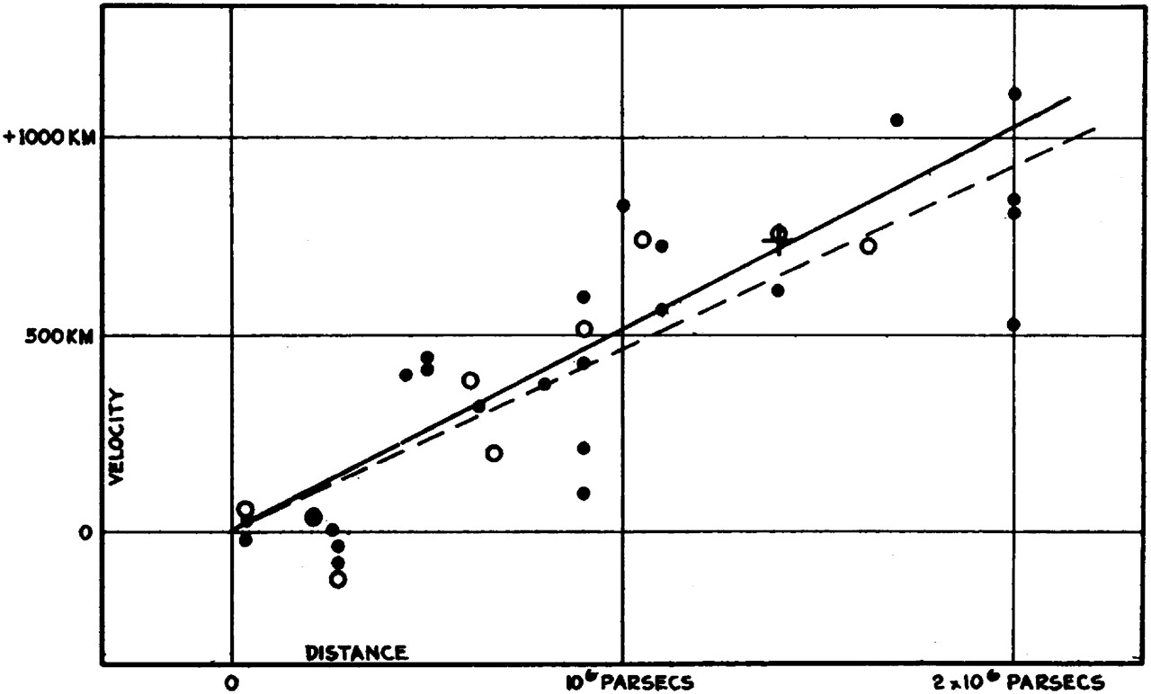
In 1929 Edwin Hubble put out an article with the distances and relative velocities of a few dozen galaxies he and his assistant Milton Humason had measured combined in a plot that was to make history (fig. 1(c)). These results were however much less simple to obtain than the previous statement would suggest, just like its interpretation into the present model of cosmology took decades to be established.

(c) Velocity to distance correlation of Galaxies (y axis is km/s). Hubble, E. P. (1929) Proc. Natl. Acad. Sci. USA 15, 168–173, full text

(d) Modern day version of Hubble diagram (with swapped axes) from Betoule et al.

Figure 2: Original and current Hubble diagram.

When Hubble started his research, these galaxies were not even thought to be so, part of the scientific community believed they were nebulae within the Milky Way, which gives an idea of how little was known about distances at the turn of the twentieth century. The confusion was there for several reasons, for one the poor resolution of the instruments made them appear as cloudy patches in the sky. Indeed one can, in an exceptionally clear night far away from any artificial light, spot Andromeda with the naked eye but it will not look much like a galaxy, just a hazy spot of faint light. This type of objects had been catalogued in the eighteen century when in 1771 Charles Messier published Nebulae and Star Clusters. Its intent was basically to mark the place of these uninteresting objects so they would not get in the way of identifying the more relevant comets that were sought for at the time. There are some hundred objects in this catalogue, which is still used as reference today (Andromeda is Messier 31 or M31 for short) and as we now know, although they might look similar with low resolution, a third of them are galaxies while the rest are actual nebulae.

To find out the distances of these objects, Hubble used the 100 inch telescope at Mt Wilson Observatory in California to observe them each for a prolonged period. In this way he was able to identify Cepheid stars within them. These are stars whose luminosity varies periodically with a frequency known to be tightly correlated with absolute luminosity (the power or how much light the star produces per unit time). By measuring their apparent luminosity, that is how much light reaches us, one can work out how far the star is by how diluted the power seems. In this way Hubble estimated that M31 (Andromeda) was 300 kpc away. The size of the Milky way had just recently been determined by the work of Harlow Shapley around 1920 to be $\sim 30$ kpc so this result showed that these formations where well outside the Milky way.

For the other axis of the plot in fig. 1(c) one needs relative velocity to us. In order to find this out one can use the spectrum instead of the intensity of the light reaching us. Spectral emission lines from common elements we can at times compute from first principles as with Hydrogen or simply and to more accuracy measure them here in the laboratory. Then when looking at the spectrum of light from a galaxy one can identify emission lines and hence deduce information about the elements making up its composition. For example we know that the transition between the two hyperfine split 1S states of Hydrogen has a wavelength of 21 cm. These spectral lines however do not sit exactly on top of the ones we measure here on earth but are displaced up or down. This up or down is actually given a name, if the line appears of higher frequency (smaller wavelength) we say it is blue shifted whereas if is of lower frequency (longer wavelength) it is red shifted. As you might have guessed the naming comes from the visible spectrum of light and its ultraviolet and infrared limits.

The reason for this shift is the relative velocity to us in an phenomenon dubbed Doppler effect. This is the effect that makes ambulances approaching sound at a higher pitch than those going away. In astronomy Vesto Slypher had already made use of this effect to estimate distances and Hubble employed the same methodology. The relation between the spectrum displacement and the relative velocity is given as

$z={\displaystyle \frac{{\nu }_{\mathrm{emit}}}{{\nu }_{\mathrm{obs}}}}-1={\displaystyle \frac{{\lambda }_{\mathrm{obs}}}{{\lambda }_{\mathrm{emit}}}}-1\simeq {\displaystyle \frac{v}{c}}$ (1.1)

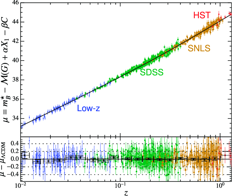
where $z$ is called the redshift and the last equality holds in the non-relativistic limit, where all the data that Hubble took falls in. Finally with these two sets of data Hubble put together the plot of fig. 1(c). It is not perhaps a very convincing linear correlation yet the present day version of the plot to the right 1(d) should convince the sceptics.

The slope of the linear correlation is called the Hubble rate $H_0$ with a 0 subindex to mark it is measured today, again because it was not the same in the past, numerically it is parametrized as

$H_0=100\times \left(h\right){\displaystyle \frac{\mathrm{km}}{\mathrm{s}}}{\displaystyle \frac{1}{\mathrm{Mpc}}}\stackrel{[4]}{=}100\times \left(0.67\pm 0.01\right){\displaystyle \frac{\mathrm{km}}{\mathrm{s}}}{\displaystyle \frac{1}{\mathrm{Mpc}}}$ (1.2)

where we took the value for $h$ from [2] in the second line but given that this value differs notably when taken from other sources it is common leave $h$ unspecified (to avoid confusion with Planck constant here we will only use $\mathrm{\hslash }$). This linear correlation tells us that velocity is proportional to distance $v=H_{0}d$ i.e. that galaxies are receding from us and faster the furthest away. We will elaborate on the simple consequences of this in the end of this lecture, for now let’s review the other main piece of evidence for modern cosmology.

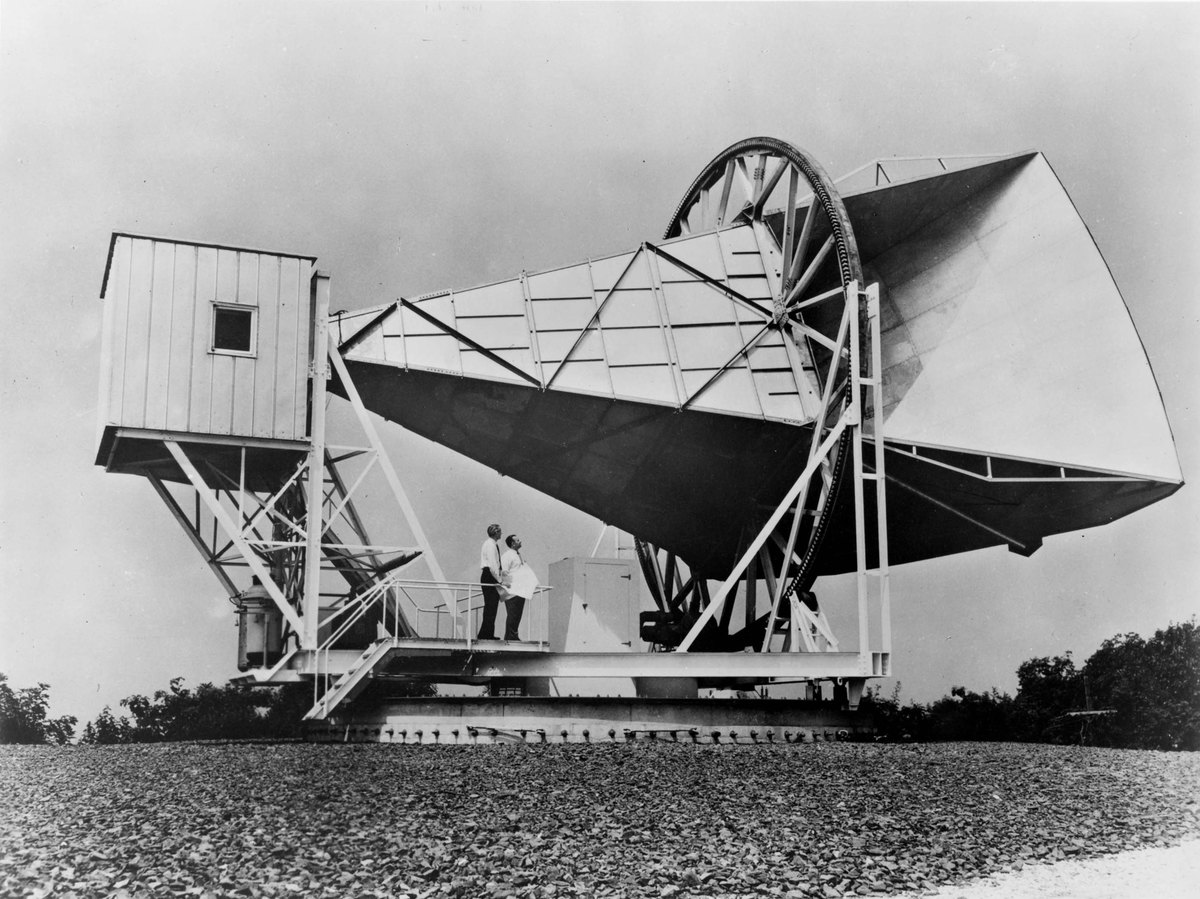
1.2 Cosmic Microwave Background

Back in the 1960s Arno Penzias and Robert Wilson were given access to a giant horn antenna designed to detect microwaves at Bell Telephone Laboratory. The original purpose of the antenna was to receive radiation from the Echo satellite in an early commercial test of satellite communications. The project was however done by 1964 and Penzias and Wilson were given control of the antenna to study cosmic microwave light. Microwave light has a wavelength from around milimeter to meter size and Penzias and Wilson started looking at the wavelengths around 7 cm . As in any experiment one of the first steps is to study systematic errors in the apparatus. There was a background noise getting in the way of their experiment which they tried to pin down for a year. They tested for this noise coming from the electronics of the equipment by cooling it, for radiation in the atmosphere by pointing the antenna in different directions, and even evacuated nesting pigeons and cleaned their mess. None of these seemed to account for this static, this noise, yet at least this revealed the noise was isotropic, i.e. coming with equal intensity from all directions in the sky and hence likely of extra-galactic origin.

Still they hesitated to put out their results up until a fateful phone call. In conversation with a colleague and when asked about how his work was going with the antenna Penzias replied that everything was well except for part of the results they did not understand. His colleague then recalled that he had been told by another colleague of a talk given by P. J. Peebles about some cosmic radiation coming from the early stages of the universe evolution and by now redshifted into the microwave range. The prediction actually predates the work of Peebles and his colleague Dicke and was first posed by Ralph Alpher and Robert Herman in 1948 although the former did not know about the latter.

Penzias and Wilson got in contact with Peebles and two papers were produced and sent to the Astrophysical Journal, one by Penzias and Wilson presenting the results (but cautious not to stipulate on the cause of the noise other than a mention to a companion paper) and another by Peeble, Dicke, Roll, and Wilkinson interpreting the result in terms of the cosmological big bang theory. We today call this isotropic cosmic noise the microwave Cosmic Microwave Background (CMB) and is one of the pillars of observational cosmology.

(a) Penzias, Wilson and the Horn antenna.

(b) CMB spectrum from COBE

Figure 3: The cosmic microwave background

There is a wealth of data to be found in the CMB, for now what is relevant to underline is the shape of this spectrum. This can be seen in fig. 2(b) where experimental data is superimposed with prediction. The prediction is that of black body radiation, the shame shape that one would get on the inside of a hermetic furnace in equilibrium. The distinctive feature of this type of radiation is that the shape depends only on one parameter, the temperature $T$. In particular the expression for the intensity as a function of radiation frequency reads

$I(\nu )={\displaystyle \frac{4\pi {\nu }^3}{e^{2\pi \nu \mathrm{\hslash }/k_{B}T}-1}}$ (1.3)

where $k_B$ is Boltzmann constant, $k_B=8.617\times {10}^{-5}$ eV/K with K degree Kelvin and $\mathrm{\hslash }$ Plancks reduced constant $\mathrm{\hslash }=6.582\times {10}^{-16}$eVs. The fit is staggeringly accurate as shown in fig. 2(b); it is in fact the most ideal black body radiation we have ever observed. The associated temperature that one can extract from this plot is

$T_0$ $=2.725\text{ Kelvin}$ CMB temperature today (1.4)

1.3 The early universe

Let us finally put together these two experimental findings. First from Hubble’s discovery one has that if at cosmic distances everything is moving away from us, things used to be much closer and we can estimate when.

Take any galaxy at a distance $d$ from us, one has, naively extrapolating its velocity to be the same in time, that if it is moving away at a velocity $v$, it used to be next to us some time $t$ ago

$t={\displaystyle \frac{d}{v}}={\displaystyle \frac{d}{H_{0}d}}={\displaystyle \frac{1}{H_0}}$ (1.5)

where in the second equality we have just substituted in Hubble’s law. The distance, the one label that the galaxy we chose had, drops out of the equation; this means that this time $t$ is the same for any galaxy. Roughly all of the known cosmos used to be clumped together a time $1/H_0$ ago! What is this time if we convert (1.2) into years? The current estimate for the age of the universe is 14 thousand million years, how does it compare with the naive estimate?

If one takes this conclusion further, when all the matter in the known universe was compressed together the energy per unit volume of the system must have been exceedingly large, just as a gas heats up when compressed. In fact if the universe had been hot enough, atoms would have ‘melted’, the electrons would be stripped away from the nucleus and for higher temperatures nuclei would have dissociated into neutrons and protons. Implicit in this discussion of a hot universe there is of course temperature.

Well we have already talked about temperature, but in the context of the microwave radiation discovered by Penzias and Wilson. Although this talk of temperature was simply used to characterize the radiation, it probed to be a temperature that we can trace back to this hot and dense initial universe; whereas electrons and nucleons have undergone processing since the early universe to appear as intergalactic gas or galaxies themselves, the light from this early universe has travelled undisturbed to reach us today. Not only that but the fact that the spectrum follows so closely the shape of a black body tells us that the early universe was in nearly perfect equilibrium.

These are the two basic concepts that thread through most of cosmology and whose balance accounts for much of the events in cosmological history: (i) the universe is expanding (ii) in its early stage it used to be in thermal equilibrium with temperature $T$.

Problems

I Let’s do some units conversion; from next chapter on, we will use natural units $\mathrm{\hslash }=c=k_B=1$ in our formulae to reduce the number of letters in them. However we will want to restore powers of these constants to express final quantities in e.g. cm, years or Kelvin. So inserting powers of $\mathrm{\hslash },c,k_B$ calculate:

$H_0^{-1}$ in years $H_0^{-1}$ in parsecs $T_0$ in eV $T_0^3$ ${\text{in cm}}^{-3}$ (1.6)

II Deduce Doppler’s shift for the relativistic case to find

$z=$ $\sqrt{{\displaystyle \frac{1+v/c}{1-v/c}}}-1$ $v>0\text{ for receeding emitter}$ (1.7)

[Hint: In the emitter frame the ‘crests’ of the wave are emitted every $1/\nu$ seconds and so a distance apart (= wavelength) $c/\nu$, convert this time interval $1/\nu$ to the observer frame to find the distance between crests she sees]. Looking at data on in fig. 2(a), is the non-relativistic approximation justified? On fig. 2(b), looking at the horizontal axis is it still?

2 Homogeneous & Isotropic

The Hubble diagram did not break down galaxies by where in the sky they were located; whether the galaxy one is looking at is in the direction of Cassiopeia or in the vicinity of the Southern Cross, they all follow the same law for their velocity vs distance. Furthermore one would roughly find the same number of galaxies looking into a fixed-size solid angle in any part of the sky. This is to say that the universe seems isotropic, the same in all directions at cosmological scales. It is also homogenous on these scales.

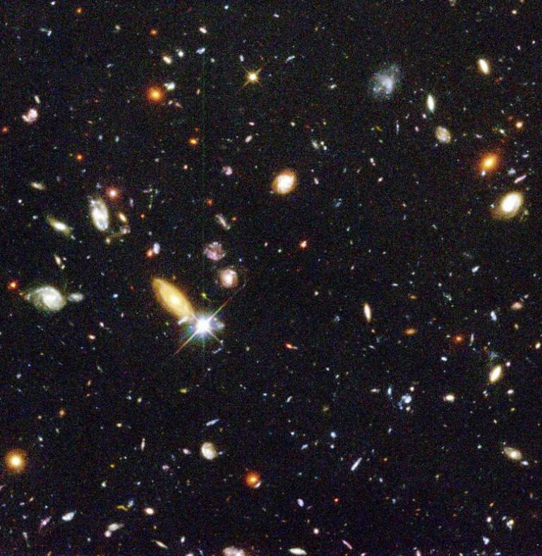
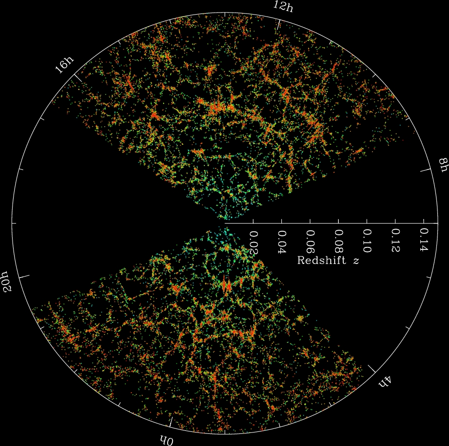
A theory argument to arrive at an homogeneous universe from an isotropic one is to assume our place in it is not special (a.k.a. cosmological principle); if a universe looks the same from any point of reference it must be homogeneous too. One need not rely on theory however, measuring distances of galaxies from us and their angular coordinates in the sky we can create a map, which is what galaxy surveys do. The size of this ‘census’ is quite formidable, as an example the Sloan Digital Sky Survey has mapped nearly a million galaxies and figure 1(a) shows a 2d slice of the map that the experiment produced.

This homogeneity and isotropy seems counter-intuitive from the human or even astrophysical perspective; right where we are there seems to be a lot of matter around whereas if one goes a few tenths of thousand light years out there is comparatively nothing. The answer to this is two-fold. First one should remember what our ruler is in cosmology; consider water, it does seem to us humans homogeneous yet we know at a microscopic level it is not a continuum but it is made of molecules and space between them. Similarly with cosmology there are as many galaxies in a few dozen megaparsec-side box around us as in the box next to it. Secondly what we ‘see’ is far from all there is; as the dynamics will reveal in two lectures time, the weight of galaxies is negligible, a mere $0.5\%$ of the total energy density. Even within visible matter, galaxies constitute $10\%$ of the whole with the majority being intergalactic dust. The use we will find for galaxies is as probes into the cosmological expansion (tracers) with negligible effect (back-reaction) on the dynamics.

Before moving on to codify this homogeneity and isotropy mathematically, it is worth pondering for a minute the fact that the universe is so ‘simple’ at the largest scale when it needed not be so. It is indeed a clue to early-time dynamics, but we do not yet have the tools to explore this. Let us then for now embrace this happy circumstance that will simplify the mathematics for us.

2.1 The metric

The previous lecture gave the evidence for an expanding universe where, we have just learned, no point is special. Therefore the distance $\mathrm{\ell }$ between any two given points, let us take them to be two distant galaxies, will grow with time. We describe this effect by introducing the scale factor $a(t)$ as

$\mathrm{\ell }=a(t)|\mathrm{\Delta }\underset{¯}{x}|$ (2.1)

where $\mathrm{\ell }$ is the physical distance, $\mathrm{\Delta }x={\underset{¯}{x}}_A-{\underset{¯}{x}}_B$ with ${\underset{¯}{x}}_A=(x_A^1,x_A^2,x_A^3)$, ${|\mathrm{\Delta }\underset{¯}{x}|}^2={(\mathrm{\Delta }{x}^i)}^2$ and we have used $a$ to ‘factor out’ time from a space like variable $\underset{¯}{x}$. There is some ambiguity in this splitting of distance into $x$ and $a$ as happens when one defines a physical quantity in terms of two constructs, so let us for practical purposes normalize. We take $|\mathrm{\Delta }x|$ to be physical distances as measured today ($t_0$)

$|\mathrm{\Delta }x|$ $\equiv \mathrm{\ell }(t_0)$ $a(t_0)$ $=1$ (2.2)

where the zero index denotes present time, for reference $t_0=13.9$ thousand million years. Lastly to implement the rate of expansion as measured in the Hubble law one has

${\displaystyle \frac{d\mathrm{\ell }(t)}{dt}}$ $={\displaystyle \frac{d(a(t)|\mathrm{\Delta }x|)}{dt}}={\displaystyle \frac{da}{dt}}{\displaystyle \frac{\mathrm{\ell }}{a(t)}}=H(t)\mathrm{\ell }$ $H(t)$ $={\displaystyle \frac{1}{a(t)}}{\displaystyle \frac{da(t)}{dt}}$ (2.3)

This gives $H$ in terms of the scale factor and presents us with the Hubble rate $H$ as the growth relative to the current size. In other words the inverse of $H$ gives the time scale that takes for the universe to double in size. You can go back to eq. (1.2) for the value of Hubble today and check how much time this would take. The value of $H_0$ together with the convention eq. (2.2) gives the scale factor and its first derivative today, these are the final (rather than initial in this case) conditions that we will later evolve back in time with the dynamics of general relativity.

The exercise above has informally set a coordinate system, $x^{\mu }=(t,\underset{¯}{x})$ convenient to describe inertial observers caught in the expansion; a 4-dimensional trajectory in $x^{\mu }$ of one such observer is $(t,0,0,1$Mpc). One need then only specify the ‘label’ $\underset{¯}{x}$ which stays constant (and remeber corresponds to physical distance today) whilst all such observers would agree on the time coordinate, defining a common ‘clock’ ticking at the same rate. This coordinate system can of course be used to describe any other trajectory and indeed not all galaxies adjust exactly to the Hubble law; Andromeda is moving towards us so we would have $d{\underset{¯}{x}}_{\mathrm{Andromeda}}/dt\ne 0$. We call $\underset{¯}{x}$ co-moving coordinate and we say Andromeda has co-moving velocity. We will nonetheless neglect this type of effect in the following.

Figure 4: In our coordinate system galaxies stay at constant $\underset{¯}{x}$ yet distance grows.

The system above is useful for its concreteness while capturing the experimental evidence yet it is important to realize it is a conventional choice. One could multiply by inverse factors $a$ and $\underset{¯}{x}$, $a\to Ca$ $\underset{¯}{x}\to \underset{¯}{x}/C$ and the physical distance would stay the same, or one could prefer a boosted frame or change to a different time variable. These would all be different ways to describe the same system, the same physics on which every observer should agree. Although this statement sounds just as sensible as it sounds vague it does have a mathematical rewriting based on invariants. Invariants are observables whose measure would yield the same value for every observer. The first instance of this we encounter is related to space-time distance, the 4-dimensional line element:

$d{s}^2=d{t}^2-a{(t)}^{2}d{\underset{¯}{x}}^2=d{t}^2-a{(t)}^2(d{r}^2+r^2(d{\theta }^2+\sin {(\theta )}^{2}d{\varphi }^2))=g_{\mu \nu }d{x}^{\mu }d{x}^{\nu }$ (2.4)

with $d$ being a differential, the infinitesimal version of $\mathrm{\Delta }$, and $g_{\mu \nu }$ is the metric, the link between our coordinate system and physical space-time distances. Already above one has a change of variables; albeit a familiar one, it does serve to illustrate that what we call the metric is different in each frame

$g_{\mu \nu }$ $x^{\mu }=$ $(t,x^1,x^2,x^3)$ (2.5)

$g_{\mu \nu }$ ${(x^{\prime })}^{\mu }=$ $(t,r,\theta ,\varphi )$ (2.6)

The connection with distances as we have discussed them initially can be obtained as the difference of two space-time points $\mathrm{\Delta }{x}^{\mu }=x_a^{\mu }-x_b^{\mu }=(0,{\underset{¯}{x}}_a-{\underset{¯}{x}}_b)$, ${\mathrm{\ell }}^2=-g_{\mu \nu }\mathrm{\Delta }{x}^{\mu }\mathrm{\Delta }{x}^{\nu }$.

Curvature
Thus far, for the sake of introducing one concept at a time, we have kept an implicit euclidean geometry in the 3 space coordinates. This need not be the case and the differential geometry language of metrics allows for a simple implementation of deviations from the ‘flat’ case.

Indeed the metric $g_{\mu \nu }$ could be a function of space and not only time. It cannot be however an arbitrary function of space given the requirement of homogeneity and isotropy; if space is not flat and has some curvature it must be the same everywhere and in every direction. One such geometric object is the sphere (although the one we can visualize is two dimensional), so to incorporate the effects of curvature into a metric let us first contemplate the case of positive curvature or spherical geometry. This is perhaps easiest if one goes to a one-extra-dimension Euclidean space and defines our space as a hyper-surface. This means a metric and constraint as:

${(x_4)}^2+{\underset{¯}{x}}^2$ $={\text{R}}_{\text{U}}^2$ $d{\mathrm{\ell }}^2$ $=d{x}_4^2+d{\underset{¯}{x}}^2$ (2.7)

where $x_4$ is an artificial extra dimension that we promptly dispose of by solving for $x_4$ as $x_4(\underset{¯}{x})$ and substituting back in the metric to obtain

${\displaystyle \frac{{(\underset{¯}{x}\cdot d\underset{¯}{x})}^2}{{\text{R}}_{\text{U}}^2-{\underset{¯}{x}}^2}}+d{\underset{¯}{x}}^2={\displaystyle \frac{d{r}^2}{1-r^2/{\text{R}}_{\text{U}}^2}}+r^2(d{\theta }^2+\sin {(\theta )}^{2}d{\varphi }^2)$ (2.8)

with $r=|\underset{¯}{x}|$. One has therefore that distances in the $\theta ,\varphi$ direction are as in flat space, yet the $r$ direction has an $r$-dependent factor. Despite the appearances the point $r=0$ is in no way special and has the same curvature as any other.

The same exercise can be repeated for negative curvature with a Minkowskian metric

$-{(x_4)}^2+{\underset{¯}{x}}^2$ $=-{\text{R}}_{\text{U}}^2$ $d{s}^2$ $=-d{x}_4^2+d{\underset{¯}{x}}^2$ (2.9)

to obtain instead

$-{\displaystyle \frac{{(\underset{¯}{x}\cdot d\underset{¯}{x})}^2}{{\text{R}}_{\text{U}}^2+{\underset{¯}{x}}^2}}+d{\underset{¯}{x}}^2={\displaystyle \frac{d{r}^2}{1+r^2/{\text{R}}_{\text{U}}^2}}+r^2(d{\theta }^2+\sin {(\theta )}^{2}d{\varphi }^2)$ (2.10)

Although the math is straight forward and a natural extension of the positive curvature case, the non-positive metric makes this case harder to visualize. Standard 2 dimensional surfaces to convey the three possibilities for curvature are sketched in fig. 5.

Figure 5: Negative, null and positive curvature surfaces.

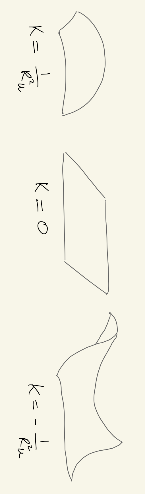
The previous results can be synthesized in the line elements

$d{s}^2$ $=d{t}^2-a{(t)}^2({\displaystyle \frac{d{r}^2}{1-K{r}^2}}+r^2(d{\theta }^2+\sin {(\theta )}^{2}d{\varphi }^2))$ $K$ $=\{\begin{array}{c}\hfill {\displaystyle \frac{1}{{\text{R}}_{\text{U}}^2}}\hfill \\ \hfill 0\hfill \\ \hfill -{\displaystyle \frac{1}{{\text{R}}_{\text{U}}^2}}\hfill \end{array}$ (2.11)

the three cases are referred to as positive curvature or closed universe $K>0$, flat universe $K=0$, and negative curvature or open universe . In order to extend the co-moving distance concept to the curved case we perform a change of variables from $r$ to $\chi$ as

$d{s}^2=d{t}^2-a{(t)}^2(d{\chi }^2+S_K^2(\chi )(d{\theta }^2+\sin {(\theta )}^{2}d{\varphi }^2))$ $S_K(\chi )=$ $\{\begin{array}{c}\hfill {\text{R}}_{\text{U}}\sin (\chi /{\text{R}}_{\text{U}})\hfill \\ \hfill \chi \hfill \\ \hfill {\text{R}}_{\text{U}}\sinh (\chi /{\text{R}}_{\text{U}})\hfill \end{array}$ (2.12)

In this way co-moving distance and physical distance keeps the linear relation so $\mathrm{\ell }=a\mathrm{\Delta }x$ now reads $\mathrm{\ell }=a\mathrm{\Delta }\chi$. Also note that the $R\to \mathrm{\infty }$ limit returns a flat geometry as it should.

This metric, known as Friedman Robertson Walker, is the most general one adhering to the homogeneity and isotropy assumptions and is described by one function of time and a constant ${\text{R}}_{\text{U}}$ for the curvature of 3 space. Simple as it might seem it is worth spending some time familiarizing oneself with it which is what we do next.

2.2 The path of light

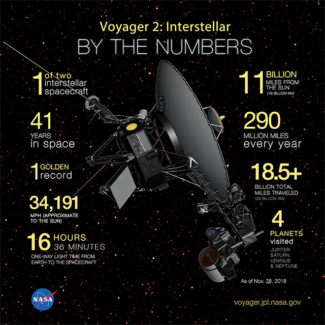
How does one turn observations into data in our coordinate system? First note the rather obvious yet unavoidable fact that we are very much stuck in the same place for cosmological observations; even the further distances we have sent missions to are negligible in cosmology. We therefore rely on information reaching earth from far away. The information available at present comes overwhelmingly in the form of light, yet we have also ‘seen’ the cosmos through neutrinos and more recently gravitational waves. All these are the fastest means possible of transmission since photons and gravitons travel at the speed of light and neutrinos nearly so. Let us then examine how waves of massless particles, be it light or gravity waves, propagate in our coordinate system.

The statement of the speed of light being the same for all observers translates into the defining equation for the invariant line element of the trajectory of light:

$(t(\sigma )$ $,\underset{¯}{x}(\sigma ))\mathit{\hspace{1em}}\mathrm{light}\mathrm{trajectory}$ $ds{(\sigma )}^2$ $=0$ (2.13)

Let us for simplicity assume a radial ray of light in the coordinate system of eq. (2.12) to write it explicitly as

$ds{(\sigma )}^2$ $=\left[{\left({\displaystyle \frac{dt}{d\sigma }}\right)}^2-a{(t(\sigma ))}^2{\left({\displaystyle \frac{d\chi }{d\sigma }}\right)}^2\right]{(d\sigma )}^2=0$ $\Rightarrow \mathit{\hspace{1em}}dt$ $=\pm a(t)d\chi$ (2.14)

With this much input and without solving for $\sigma$ one can already ask questions; the first one we pose is how far has light emitted some time $\mathrm{\Delta }t=t_0-t$ ago travelled to reach us? The answer is

$\mathrm{\ell }(t)={\displaystyle \int 𝑑\mathrm{\ell }}={\displaystyle \int a(t)𝑑\chi }={\displaystyle \int 𝑑t}=c(t_0-t)$ (2.15)

where we momentarily restored the speed of light in our equation. The result is then that light travels a physical distance equal to the time interval $\mathrm{\Delta }t$ in our frame (times the speed of light). If we ask instead what is the co-moving distance (equal to physical distance today) to the object that emitted that light we find

$\mathrm{\Delta }\chi ={\displaystyle \int 𝑑\chi }={\displaystyle {\int }_t^{t_0}}{\displaystyle \frac{dt}{a(t)}}$ (2.16)

which one cannot compute unless we are given the form of $a(t)$.

Figure 6: Time (t) vs distance (d) for the path of a photon from a distant galaxy.

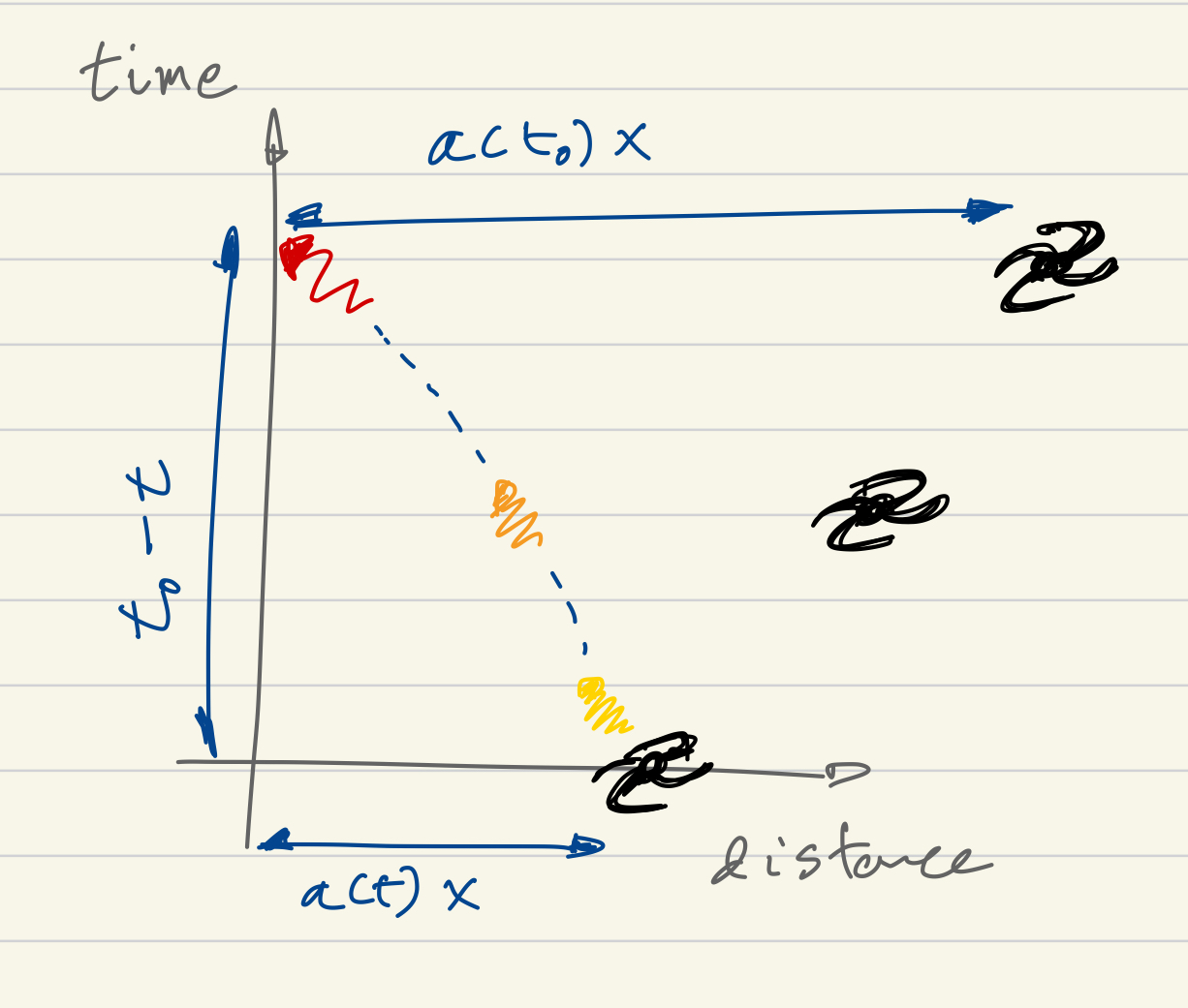
What we can conclude nonetheless, if the universe has been expanding ever since $t$, is that one distance is greater than the other $\mathrm{\Delta }{\chi }_{\mathrm{light}}>\mathrm{\Delta }{\mathrm{\ell }}_{\mathrm{light}}$. This is simple to understand; light takes some time to travel, at the time when light was emitted the universe was smaller and the emitter is farther today than it was at time $t$. This is also the case in Minkowski space-time for inertial observers moving away from each other. Nevertheless our case is not Minkowski and it should differ from it. This is relevant to realize because one could naively picture the expansion of the universe as an ‘explosion’ where fragments are moving away from each other but in otherwise an special relativity background. If this were true the distance light would have travelled is simply the distance of the object from us at the time of emission. This distance at time $t$ one can obtain from the co-moving distance by rescaling with $a(t)/a(t_0)$. It then follows (given a monotonically increasing $a(t)$) :

$\mathrm{distance}\mathrm{at}\mathrm{emission}$ $=a(t){\displaystyle {\int }_t^{t_0}}{\displaystyle \frac{d{t}^{\prime }}{a(t^{\prime })}}$

$\mathrm{distance}\mathrm{travelled}\mathrm{by}\mathrm{light}$ $={\displaystyle {\int }_t^{t_0}}𝑑t^{\prime }$

$a(t){\displaystyle {\int }_t^{t_0}}{\displaystyle \frac{d{t}^{\prime }}{a(t^{\prime })}}$ (2.17)

with . That is, from the first inequality (distance at the time of emission) (distance travelled) . Space itself has expanded in the intervening time $\mathrm{\Delta }t$!

2.3 Measuring distance

As outlined in the previous lecture there are a number of methods for determining distances in cosmology, our coordinate system allows to put together all different measurements into coordinates and compare them. We next outline two methods of distance determination and what co-moving coordinates they correspond to.

Luminosity distance. Some astrophysical objects have a known luminosity (energy emitted per unit time in the form of light), which one can compare with how much energy in radiation reaches the area of our detector per unit time.

The energy emitted will dilute into a shell around the emission point of radius, today, $a(t_0)\chi =\chi$. The area of this shell depends on the geometry; a positive geometry will have, for given $\chi$, an area smaller than the flat case $4\pi {\chi }^2$. Exercises for circles instead of spheres with a pen, an orange and peeling will convince the dubious. Conversely the negatively curved case has a larger area than $4\pi {\chi }^2$. The area in the curved case can be computed realizing that $\chi /{\text{R}}_{\text{U}}$ acts as the polar angle in our 3d sphere and a flat slice though our constant $\chi$ surface has radius ${\text{R}}_{\text{U}}\sin (\chi /{\text{R}}_{\text{U}})$ in the hyper-plane. The three possibilities read:

$A=4\pi \{\begin{array}{c}\hfill {\text{R}}_{\text{U}}^2{\sin }^2(\chi /{\text{R}}_{\text{U}})\hfill \\ \hfill {\chi }^2\hfill \\ \hfill {\text{R}}_{\text{U}}^2{\sinh }^2(\chi /{\text{R}}_{\text{U}})\hfill \end{array}=4\pi S_K^2$ (2.18)

In addition to this effect one has that the rate at which one receives photons is dilated with respect to the rate of emission whereas the energy of an individual photon, proportional to the frequency, also diminishes with the expansion of the universe. This last point we will demonstrate explicitly in the next chapter; intuitively it is a consequence of the stretching of space and the energy of a photon being inversely proportional to the wavelength $E\propto 1/\lambda$. All in all the flux we observe on earth related to the luminosity $L$ is

$F={\displaystyle \frac{a{(t)}^{2}L}{4\pi S_K^2(\chi )}}\equiv$ ${\displaystyle \frac{L}{4\pi d_L^2}}$ (2.19)

where we have defined the luminosity distance $d_L$ as it is conventional. This equation which can be inverted to find $\chi$. One has then that the same star seems dimer in an open universe and brighter in a closed one.

Figure 7: Trigonometry on a sphere

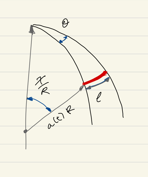
Angular distance. Another possibility is looking at objects whose dimensions are known together with trigonometry. Note that angles do not change in time for an homogeneously and isotropically expanding universe but they stay the same. For simplicity consider a unidimensional rod of length $l$ laid perpendicular to the line of sight at a distance much greater than its size so that the angle $\theta \ll 1$ in radians.

Tracing time back to when the light reaching us was emitted, the object was at a distance $a(t)\chi$ (co-moving distance scaled back). The relation to the length $l$ is then given by trigonometry in curved space. For the flat case a simple sketch leads to the relation $\theta a(t)\chi =l$. The positive curvature case takes a bit more sketching, although the derivation for luminosity distance above offers clues. The co-moving coordinate over $R$ gives the polar angle whose sine gives the distance to the axis at $\chi =0$. This is sketched in fig. 7 and leads to the relation $a(t)R\sin (\chi /R)\theta =l$. This generalizes to the expression

$l=a(t)S_K(\chi )\theta \equiv d_A\theta$ (2.20)

One has then that the same object at the same distance $\chi$ from subtends and angle

$\theta ={\displaystyle \frac{l}{a(t)}}\{\begin{array}{c}\hfill {({\text{R}}_{\text{U}}\sin (\chi /{\text{R}}_{\text{U}}))}^{-1}\hfill \\ \hfill {\chi }^{-1}\hfill \\ \hfill {({\text{R}}_{\text{U}}\sinh (\chi /{\text{R}}_{\text{U}}))}^{-1}\hfill \end{array}$ (2.21)

That means, since objects seem larger (larger $\theta$) in a positive curvature space and smaller in a negative curvature one. To get a sense of why this is the case intuitively you can think of a sphere with the observer in the north pole and the object south of the equator.

If one knows both the luminosity and dimensions of an object, extracting $\chi$ from both methods above provides a useful consistency check. Let us collect here both definitions

$d_L=$ $\sqrt{{\displaystyle \frac{L}{4\pi F}}}={\displaystyle \frac{S_K(\chi )}{a(t)}}$ $d_A$ $={\displaystyle \frac{l}{\theta }}=a(t)S_K(\chi )$ (2.22)

where $\chi$ itself can be written as a function of the emission time $t$ as in eq. (2.16)

Problems

I The change of variables $r(\chi )$ from equation (2.11) to (2.12) satisfies, by comparing the two equations,

$d\chi ={\displaystyle \frac{dr}{\sqrt{1-K{r}^2}}}$ (2.23)

Solve this relation with $r(0)=0$ for the three values of $K$. How is the expression you found related to $S_K(\chi )$?

II Given the scale factor $a(t)={(t/t_0)}^{2/3}$ compute the physical distance $\mathrm{\ell }(t)$ light travels from $t$ to $t_0$ (2.15), the co-moving distance $\mathrm{\Delta }\chi$ (2.16) and distance at emission $a(t)\mathrm{\Delta }\chi$. Is relation 2.2 satisfied? You can check by taking $t=t_0/2$ for instance.

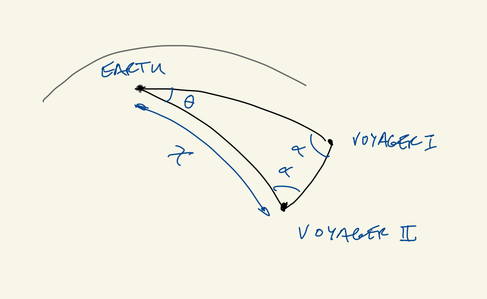
III Use the two voyager missions and the earth for a determination of the universe geometry via trigonometry. Assume the two missions are the same distance $\chi$ away from us today using data on the figure (careful this is NASA so billion=${10}^9$), the line-of-sight of the two form a relative angle $\theta$ as seen from earth whereas on board the angle between earth and the other spacecraft is $\alpha$, and take a spherical geometry for your computations. Determine $\alpha$ in terms of $\chi ,\theta ,R$ to be:

$\cos (\alpha )={\displaystyle \frac{\sin (\theta /2)\cos (\chi /{\text{R}}_{\text{U}})}{\sqrt{1-{\sin }^2(\theta /2){\sin }^2(\chi /{\text{R}}_{\text{U}})}}}$ (2.24)

Expand on $\chi /R$ and assuming we measure angles with ${10}^{-16}$ degree accuracy, find a bound on ${\text{R}}_{\text{U}}$.

3 Geodesics, Horizons & Redshift

The previous lecture laid out the metric used in cosmology and connected it to observations. In particular the scale factor measuring the growth of the universe has a first derivative related to the Hubble rate as $a^{\prime }/a=H_0$ today and we set $a(t_0)=1$ so that co-moving distance $|\chi |$ is present time physical distance. An additional parameter of the metric accounted for a possible curvature of space, $K$, whose current experimental value is compatible with 0 but we keep general for now.

3.1 Geodesics

Although no reference to gravity has been made so far, the metric incorporates all its effects to the homogenous and isotropic approximation we are taking here. This will be made explicit in the next lecture when the equations of general relativity show how matter sources the dynamics of the metric. For now this section studies the motion of test particles or probes in this background metric.

Since gravity is the single relevant interaction in the cosmological regime today the metric must suffice to determine dynamics. Let us consider a point particle of mass $m$ travelling in our FRW universe. As we did with light we describe its 4 dimensional path with one parameter $\sigma$ such that the first derivative is the 4-momentum:

$x^{\mu }$ $(\sigma )$ ${\displaystyle \frac{d{x}^{\mu }}{d\sigma }}$ $=P^{\mu }=(E,P^i)$ $g_{\mu \nu }{P}^{\mu }{P}^{\nu }$ $=m^2$ (3.1)

The path is then given by solving the equation of motion yet no force of gravity is in sight. This is so because in the geometric language of general relativity the gravitational force is in the connection or first derivative of the metric and the equation of motion is the geodesic equation or path of minimum space-time distance. Since this formulation might be unfamiliar to the reader, here first we take a detour to introduce geodesics as describing dynamics.

1.  

2. To ease us into geodesic equations and the Connection let us resort momentarily to flat space $x^i$ and the simple equation for inertial motion i.e. in the absence of any force:

   ${\displaystyle \frac{d^2{x}^i}{d{\tau }^2}}$ $=0$ $d{s}^2$ $={\delta }_{ij}d{x}^{i}d{x}^j$ (3.2)

   where ${\delta }_{ij}$ is the Kronecker delta. If one were to describe the system in other set of coordinates $y^i$,

   ${\displaystyle \frac{d}{d\tau }}\left({\displaystyle \frac{d{y}^j}{d\tau }}{\displaystyle \frac{\partial x^i}{\partial y^j}}\right)$ $=0$ $d{s}^2$ $={\displaystyle \frac{\partial x^i}{\partial y^j}}d{y}^j{\displaystyle \frac{\partial x^i}{\partial y^k}}d{y}^k\equiv g_{ij}d{y}^{j}d{y}^k$ (3.3)

   and rewrite the equations of motion (EoM) in terms of the metric $g_{ij}$, which can be done by multiplying and summing on $\partial x/\partial y$ and a little trickery

   $0=$ ${\displaystyle \frac{\partial x^i}{\partial y^l}}{\displaystyle \frac{\partial x^i}{\partial y^j}}{\displaystyle \frac{d^2{y}^j}{d{\tau }^2}}+\left[{\displaystyle \frac{\partial x^i}{\partial y^l}}{\displaystyle \frac{\partial x^i}{\partial y^j\partial y^k}}\right]{\displaystyle \frac{d{y}^j}{d\tau }}{\displaystyle \frac{d{y}^k}{d\tau }}$

   $=$ ${\displaystyle \frac{\partial x^i}{\partial y^l}}{\displaystyle \frac{\partial x^i}{\partial y^j}}{\displaystyle \frac{d^2{y}^j}{d{\tau }^2}}+{\displaystyle \frac{1}{2}}\left[{\displaystyle \frac{\partial }{\partial y^j}}{\displaystyle \frac{\partial x^i}{\partial y^l}}{\displaystyle \frac{\partial x^i}{\partial y^k}}+{\displaystyle \frac{\partial }{\partial y^k}}{\displaystyle \frac{\partial x^i}{\partial y^l}}{\displaystyle \frac{\partial x^i}{\partial y^j}}-{\displaystyle \frac{\partial }{\partial y^l}}{\displaystyle \frac{\partial x^i}{\partial y^j}}{\displaystyle \frac{\partial x^i}{\partial y^k}}\right]{\displaystyle \frac{d{y}^j}{d\tau }}{\displaystyle \frac{d{y}^k}{d\tau }}$

   $=$ $g_{lj}{\displaystyle \frac{d^2{y}^j}{d{\tau }^2}}+{\displaystyle \frac{1}{2}}\left[{\displaystyle \frac{\partial }{\partial y^j}}{g}_{kl}+{\displaystyle \frac{\partial }{\partial y^k}}{g}_{lj}-{\displaystyle \frac{\partial }{\partial y^l}}{g}_{jk}\right]{\displaystyle \frac{d{y}^j}{d\tau }}{\displaystyle \frac{d{y}^k}{d\tau }}$

   $\equiv$ $g_{lj}\left({\displaystyle \frac{d^2{y}^j}{d{\tau }^2}}+{\mathrm{\Gamma }}_{jk}^j{\displaystyle \frac{d{y}^j}{d\tau }}{\displaystyle \frac{d{y}^k}{d\tau }}\right)$ (3.4)

   we obtain a second derivative term as in the original case plus a term quadratic in first derivatives with a coefficient which we call the connection or Christoffel symbols. This fictitious force has appeared in the process of changing to another set of coordinates or observer frame. The case of gravity itself is not unlike this, one can always find a local frame in which there are no forces (the connection vanishes), a local free falling frame. Nevertheless even such an observer would be able to tell the presence of gravity by the non-vanishing second derivative of the metric through tidal forces.

 

The dynamics then will be given by the connection or first derivatives of the metric which in our case reads

$d{s}^2=d{t}^2-a{(t)}^2(d{\chi }^2+S_K^2(\chi )(d{\theta }^2+\sin {(\theta )}^{2}d{\varphi }^2))=d{t}^2-a^2(t){\widehat{g}}_{ij}d{x}^{i}d{x}^j$ (3.5)

where we have defined for convenience the internal space metric ${\widehat{g}}_{ij}=$Diag$(1,S_K^2(\chi ),S_K^2(\chi )s_{\theta }^2)$. The definition of the connection one derives from eq. (3.4) is

${\mathrm{\Gamma }}_{\nu \rho }^{\mu }={\displaystyle \frac{g^{\mu \kappa }}{2}}\left({\displaystyle \frac{\partial }{\partial x^{\nu }}}{g}_{\rho \kappa }+{\displaystyle \frac{\partial }{\partial x^{\rho }}}{g}_{\nu \kappa }-{\displaystyle \frac{\partial }{\partial x^{\kappa }}}{g}_{\nu \rho }\right)$ (3.6)

where the upper-indexes metric is the inverse as $g^{\mu \kappa }{g}_{\kappa \nu }={\delta }_{\nu }^{\mu }$.

A difference with the derivation above is that time itself is a coordinate and the geodesic equation has 4 components while the first derivative (momentum) is constrained to be on shell as in eq. (3.1). The system to be solved is then

$\left[{\displaystyle \frac{d{x}^{\nu }}{d\sigma }}{\nabla }_{\nu }\right]{\displaystyle \frac{d{x}^{\mu }}{d\sigma }}$ $={\displaystyle \frac{d{x}^{\nu }}{d\sigma }}\left({\displaystyle \frac{\partial }{\partial x^{\nu }}}{\displaystyle \frac{d{x}^{\mu }}{d\sigma }}+{\mathrm{\Gamma }}_{\nu \alpha }^{\mu }{\displaystyle \frac{d{x}^{\alpha }}{d\sigma }}\right)={\displaystyle \frac{d^2{x}^{\mu }}{d{\sigma }^2}}+{\mathrm{\Gamma }}_{\nu \alpha }^{\mu }{\displaystyle \frac{d{x}^{\nu }}{d\sigma }}{\displaystyle \frac{d{x}^{\alpha }}{d\sigma }}$ (3.7)

$g_{\mu \nu }{\displaystyle \frac{d{x}^{\mu }}{d\sigma }}{\displaystyle \frac{d{x}^{\nu }}{d\sigma }}$ $=m^2$ (3.8)

where we have introduced the covariant derivative $\nabla$ and have used the chain rule $(d{x}^{\mu }/d\sigma )\partial /\partial x^{\nu }=d/d\sigma$. The covariant derivative introduction serves more than a compact writing of the geodesic equation, it is the derivative which yields covariantly transforming objects (i.e. tensors) which one in turn needs to build the theory of gravity as the local theory of coordinate transformations. The similarity with gauge theories (as is the case of the Standard Model) which also present a covariant derivative is in fact indicative of a more profound connection between the two, yet this falls outside of our scope.

Relevant for our discussion is the fact that conservation laws which one may be used to with ordinary differentiation in the presence of gravity must be promoted, for example:

Special  Relativity General  Relativity (3.9)

${\partial }_{\mu }{J}^{\mu }$ $=0$ $\Rightarrow$ ${\nabla }_{\mu }{J}^{\mu }$ $={\partial }_{\mu }{J}^{\mu }+{\mathrm{\Gamma }}_{\mu \nu }^{\mu }{J}^{\nu }=0$ (3.10)

${\partial }_{\mu }{T}_{\nu }^{\mu }$ $=0$ $\Rightarrow$ ${\nabla }_{\mu }{T}_{\nu }^{\mu }$ $={\partial }_{\mu }{T}_{\nu }^{\mu }+{\mathrm{\Gamma }}_{\mu \alpha }^{\mu }{T}_{\nu }^{\alpha }-{\mathrm{\Gamma }}_{\mu \nu }^{\alpha }{T}_{\alpha }^{\mu }=0$ (3.11)

where we see that the covariant derivative acts on every index and with a minus relative sign on lower indices:

${\nabla }_{\mu }{A}_{\nu }={\partial }_{\nu }{A}_{\mu }-{\mathrm{\Gamma }}_{\mu \nu }^{\alpha }{A}_{\alpha }.$ (3.12)

Back to cosmology with our FRW metric differentiation and a little patience yields a connection which can be synthesised as

${\mathrm{\Gamma }}_{ij}^0$ $=a{\displaystyle \frac{\partial a}{\partial t}}{\widehat{g}}_{ij}$ ${\mathrm{\Gamma }}_{0j}^i={\mathrm{\Gamma }}_{j0}^i$ $={\displaystyle \frac{1}{a}}{\displaystyle \frac{\partial a}{\partial t}}{\delta }_j^i$ ${\mathrm{\Gamma }}_{jj}^i$ $=-{\displaystyle \frac{1}{2{\widehat{g}}_{ii}}}{\displaystyle \frac{\partial {\widehat{g}}_{jj}}{\partial x^i}}$ ${\mathrm{\Gamma }}_{ij}^i$ $={\displaystyle \frac{1}{2{\widehat{g}}_{ii}}}{\displaystyle \frac{\partial {\widehat{g}}_{ii}}{\partial x^j}}$ (3.13)

with every other element being 0. One can be more explicit and give the space-like components

${\mathrm{\Gamma }}_{\theta \theta }^{\chi }$ $=-S_{K\chi }{\displaystyle \frac{\partial S_{K\chi }}{\partial \chi }}$ ${\mathrm{\Gamma }}_{\varphi \varphi }^{\chi }$ $=-S_{K\chi }{\displaystyle \frac{\partial S_{K\chi }}{\partial \chi }}{s}_{\theta }^2$ ${\mathrm{\Gamma }}_{\varphi \varphi }^{\theta }$ $=-s_{\theta }{c}_{\theta }$ (3.14)

${\mathrm{\Gamma }}_{\theta \chi }^{\theta }$ $={\mathrm{\Gamma }}_{\chi \theta }^{\theta }={\displaystyle \frac{1}{S_{K\chi }}}{\displaystyle \frac{\partial S_{K\chi }}{\partial \chi }}$ ${\mathrm{\Gamma }}_{\varphi \chi }^{\varphi }$ $={\mathrm{\Gamma }}_{\chi \varphi }^{\varphi }={\displaystyle \frac{1}{S_{K\chi }}}{\displaystyle \frac{\partial S_{K\chi }}{\partial \chi }}$ ${\mathrm{\Gamma }}_{\varphi \theta }^{\varphi }$ $={\mathrm{\Gamma }}_{\theta \varphi }^{\varphi }={\displaystyle \frac{c_{\theta }}{s_{\theta }}}$ (3.15)

where we note that the partial derivatives are actually total derivatives $d/dt,d/d\chi$ given that the functions they act on depend only on one variable. So that finally we can write the differential equation for our trajectory in (3.1),

${\displaystyle \frac{d^2{x}^{\mu }}{d{\sigma }^2}}+{\mathrm{\Gamma }}_{\nu \rho }^{\mu }{\displaystyle \frac{d{x}^{\nu }}{d\sigma }}{\displaystyle \frac{d{x}^{\rho }}{d\sigma }}={\displaystyle \frac{d}{d\sigma }}{P}^{\mu }+{\mathrm{\Gamma }}_{\nu \rho }^{\mu }{P}^{\nu }{P}^{\rho }=0$ (3.16)

explicitly by substituting in $\mathrm{\Gamma }$. Let’s do it for the 0’th component and recalling the notation $P^{\mu }=(E,P^i)$ one finds

${\displaystyle \frac{dE}{d\sigma }}+2{\mathrm{\Gamma }}_{0i}^{0}E{P}^i+{\mathrm{\Gamma }}_{ij}^0{P}^i{P}^j={\displaystyle \frac{dt}{d\sigma }}{\displaystyle \frac{dE}{dt}}+a{\displaystyle \frac{da}{dt}}{\widehat{g}}_{ij}{P}^i{P}^j$ (3.17)

which can be turned into an equation for the energy alone by using the on-shell condition and the definition of momentum as

${\displaystyle \frac{d{x}^0}{d\sigma }}$ $={\displaystyle \frac{dt}{d\sigma }}=E$ $E^2-a^2{\widehat{g}}_{ij}{P}^i{P}^j$ $=m^2$ (3.18)

and substitution back in eq. (3.17)

$E{\displaystyle \frac{d}{dt}}E+{\displaystyle \frac{1}{a}}{\displaystyle \frac{da}{dt}}\left(E^2-m^2\right)$ $=0$ (3.19)

The ultra relativistic ($m\simeq 0$) and non-relativistic ($E\simeq m$) limits of this differential equation are simple to solve

$\mathrm{Ultra}\mathrm{Rel}.$ ${\displaystyle \frac{1}{E}}{\displaystyle \frac{dE}{dt}}-{\displaystyle \frac{1}{a}}{\displaystyle \frac{da}{dt}}$ $=0$ $E=$ ${\displaystyle \frac{a(t_i)}{a(t)}}E(t_i)$ (3.20)

$\mathrm{Non}\mathrm{Rel}.$ ${\displaystyle \frac{dE}{dt}}$ $=0$ $E=$ $m$ (3.21)

Hence we have that the energy of massless particles (e.g. light) scales inversely with the expansion of the universe while the energy of slowly moving massive particles stays the same. This result one might derive with considerably less effort just by noting that the energy of a photon is:

$E_{\text{photon}}=2\pi \mathrm{\hslash }\nu =2\pi \mathrm{\hslash }{\displaystyle \frac{c}{\lambda }}$ (3.22)

with $\nu$ and $\lambda$ frequency and wavelength respectively. If as stated in the previous lecture, space itself is expanding, wavelengths expand with it as well and this greater wavelength means smaller energy. On the other hand a point particle with mass $m$ will have a first order contribution to energy $a$ and $t$ independent.

3.2 Redshift & Horizons

The fact that the evolution of the energy in light tracks the (inverse of the) expansion of the universe allows for a simple conversion of experimental observations into dating. The first lecture outlined how the shift in the frequency of light described as the Doppler effect can be used to determine relative velocity. We can now relate this shift to the scale factor recalling the definition in eq. (1.1) which now reads:

$z=$ ${\displaystyle \frac{\nu (t)}{\nu (t_0)}}-1={\displaystyle \frac{a(t_0)}{a(t)}}-1$ $$\frac{a(t)}{a(t_0)}=\frac{1}{1+z}$$ (3.23)

Some of the furthest away objects we have seen are quasars at $z=6$ and so bring information of back when the universe was a seventh of its current size. We can even see further back to higher redshifts, only then the universe did not look anything like now; for one galaxies had not formed!

This brings us to the daring question: how far would we have to look to see the ‘birth’ of the known universe, if such a thing were possible? Recall that we obtained in the first lecture an estimate of the age of the universe by approximating when all the galaxies and everything else we see was ‘in the same place’ which is what we mean by birth. This corresponds to $a=0$ and one would expect this limit to be singular or ill defined yet the question we posed has a finite answer, in comoving distance it is:

$\eta (t_0)={\displaystyle {\int }_0^{t_0}}{\displaystyle \frac{dt}{a(t)}}$ (3.24)

where even though $a(t)\to 0$ it does so in general mildly enough so that the integral converges. This distance $\eta (t_0)$ is called the co-moving horizon today since we believe we have no way of knowing about anything beyond this radius.

However our initial scepticism about this $t\to 0$ limit is justified, it as a convenient abstraction yet we should not take it literally; the Physical laws that we know can only be taken back in time so much until the conditions of the universe are such that they break down. In the integral above however this regime makes a tiny tiny contribution to the total which is dominated by late times and for all practical purposes we can take the limit.

One can make the answer to this question time dependent to introduce what is known as conformal time:

$$\eta (t)={\int }_0^t\frac{d{t}^{\prime }}{a(t^{\prime })}$$ (3.25)

this gives the horizon at time $t$, to reiterate, the maximal co-moving distance that information about an event at $t\mathrm{=}\mathrm{0}$ can travel by time $t$. At the same time it doubles as an alternative time variable replacing $t$. The use of changing variables once more to this time $\eta$ is that causality is specially transparent to discuss in terms of $\eta$.
Causality

Consider two events occurring at times $t_1$ and $t_2$ ($>t_1$) in two different co-moving coordinate points ${\chi }_1,{\chi }_2$, let’s say for concreteness event one is a supernova explosion on a distant galaxy and event two is the decision of a scientific committee on whether to build an underground neutrino detector or not here on earth. The fastest that information from the supernova can travel is the speed of light and so by $t_2$ this information has covered a co-moving distance:

$\text{Co-moving Horizon of event 1 by time }{t}_2\mathit{\hspace{1em}\hspace{1em}}{\displaystyle {\int }_{t_1}^{t_2}}{\displaystyle \frac{dt}{a(t)}}$ $={\eta }_2-{\eta }_1$ (3.26)

Assume that the two points are far away enough so that , that is the horizon of event 1 by the time of event 2 is smaller than the distance between them. In this case information about the supernova could have not reached the committe at the time of the decision, we say the two events are causally disconnected; they couldn’t have influenced one another in any way. The light of the supernova will reach the planet later and neutrinos a bit later still, if the detector was built these would provide useful data, but they couldn’t have possibly known at the time! As history has it a number of government agencies around the world took the right decision, even if they did not have supernovas in mind, see SN 1987A.

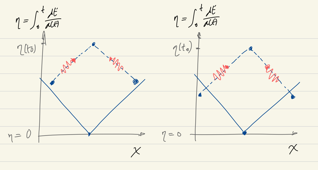
As a last discussion on causality which will be of use later, let’s consider the possible relation between events A,B in opposite directions in the sky which occurred at time $t$ and whose light is just reaching us today on earth. The fact that the light from these events is just reaching us now, if it has travelled unperturbed, means that comoving distance and comoving horizon coincide:

$|{\chi }_A-{\chi }_{us}|=|{\chi }_B-{\chi }_{us}|=\eta (t_0)-\eta (t)$ (3.27)

(in practice we can pick simultaneous events by selecting equal redshifts). Say now that the two events look strangely similar and so we ask, could they have had a common cause? The mathematical positing of this question is can they be fitted on the same light cone? Fig. 8 tries to depict the possible situations, shifting about the two simultaneous events in the presence of a vertex will convince you that the earliest the two positions could have obtained the same information is if it was emitted from the midpoint at $t=0$. By the time $t$ when the events took place the possible original signal would have covered a diameter of $2(\eta (t)-\eta (0))=2\eta (t)$ which we can compare with their distance derived from eq. 3.27

$2(\eta (t_0)-\eta (t))$ $\text{vs}\mathrm{\hspace{0.17em}\hspace{0.17em}2}\eta (t)$ (3.28)

The rather simple answer we obtain is that events that we see in opposite ends of the sky cannot be causally connected if they occurred in the first half the conformal lifetime of the universe. On the other hand when we say causally connected we mean they could have been, but they need not.

Figure 8: Events in the past causally connected LHS and disconnected RHS

Problems

I Show, given the covariant derivative action on lowered indices ${\nabla }_{\mu }{A}_{\nu }={\partial }_{\mu }{A}_{\nu }-{\mathrm{\Gamma }}_{\mu \nu }^{\alpha }{A}_{\alpha }$ that the derivative acting on the invariant object $J_{\mu }{J}^{\mu }$ satisfies

${\nabla }_{\rho }{J}^{\mu }{J}_{\mu }=({\nabla }_{\rho }{J}^{\mu })J_{\mu }+J^{\mu }({\nabla }_{\rho }{J}_{\mu })={\partial }_{\rho }(J^{\mu }{J}_{\mu })$ (3.29)

II Compute the connection elements ${\mathrm{\Gamma }}_{ij}^0$, ${\mathrm{\Gamma }}_{0j}^i$ for space-curvature-less ($K=0$) metric:

$d{s}^2=d{t}^2-a{(t)}^2({(d{x}^1)}^2+{(d{x}^2)}^2+{(d{x}^3)}^2)$ (3.30)

Check that any other element is either related by ${\mathrm{\Gamma }}_{\nu \rho }^{\mu }={\mathrm{\Gamma }}_{\rho \nu }^{\mu }$ or zero.
III Take a universe with $a={(t/t_0)}^p$ with and compute explicitly conformal time and redshift $\eta (t)$, $z(t)$. What time $t_{1/2}$ and redshift corresponds to $\eta (t_{1/2})=\eta (t_0)/2$? IV Turn eq. (3.19) into an differential equation for $dE/da$ and solve for $E(a)$ with initial conditions $E(a_i)=E_i$. If initially the energy was much above the mass $E_i\gg m$ what value of $a$ approximately sparates the regions where $E\simeq E_i{a}_i/a$ and $E\sim m$?
V Derive the geodesic equation from the variational principle applied to:

$$\int 𝑑\sigma \sqrt{g_{\mu \nu }(x(\sigma ))\frac{d{x}^{\mu }}{d\sigma }\frac{d{x}^{\nu }}{d\sigma }}$$

4 Einstein’s equations

Thus far we have taken the metric as a given, a background where we studied the evolution of light and matter, the position of our horizons and the galaxies. The metric is however dynamic and it is affected by what and how much matter is there and perturbations on the metric propagate as light does to first order.

In loose terms the dynamics of the metric will be given by an equation of motion which will contain second order derivatives, just as Maxwell’s equations contain second order derivatives of the gauge potential $A_{\mu }$. These equations of motion will not be arbitrary but admit a covariant form, like the geodesic equation. This means that the equations of motion themselves are in tensor form and obey simple transformation rules which guarantee they look formally the same to all observers.

4.1 Curvature

The covariant second-order derivative that can be built out of the metric is the Riemann tensor defined through the commutator of covariant derivatives:

$\left({\nabla }_{\mu }{\nabla }_{\nu }-{\nabla }_{\nu }{\nabla }_{\mu }\right)V^{\rho }\equiv R_{\alpha \mu \nu }^{\rho }{V}^{\alpha }$ (4.1)

which reads, in terms of the connection

$R_{\beta \mu \nu }^{\alpha }={\partial }_{\mu }{\mathrm{\Gamma }}_{\beta \nu }^{\alpha }-{\partial }_{\nu }{\mathrm{\Gamma }}_{\beta \mu }^{\alpha }+{\mathrm{\Gamma }}_{\mu \rho }^{\alpha }{\mathrm{\Gamma }}_{\beta \nu }^{\rho }-{\mathrm{\Gamma }}_{\nu \rho }^{\alpha }{\mathrm{\Gamma }}_{\beta \mu }^{\rho }$ (4.2)

The Riemann tensor is antisymmetric under exchange of the last two indices by definition but also under exchange of the first two with lowered indices $R_{\alpha \beta \mu \nu }=-R_{\beta \alpha \mu \nu }$, symmetric under exchange as $R_{\alpha \beta \mu \nu }=R_{\mu \nu \alpha \beta }$ and with a vanishing cyclic combination of the last 3 indexes $R_{\alpha \beta \mu \nu }+R_{\alpha \nu \beta \mu }+R_{\alpha \nu \mu \beta }=0$ which means that, all in all, the number of independent components is 20.

Contracting two of the indices we obtain a two-index tensor which is called the Ricci tensor:

$R_{\mu \nu }\equiv R_{\mu \alpha \nu }^{\alpha }={\partial }_{\alpha }{\mathrm{\Gamma }}_{\mu \nu }^{\alpha }-{\partial }_{\nu }{\mathrm{\Gamma }}_{\alpha \mu }^{\alpha }+{\mathrm{\Gamma }}_{\alpha \rho }^{\alpha }{\mathrm{\Gamma }}_{\mu \nu }^{\rho }-{\mathrm{\Gamma }}_{\nu \rho }^{\alpha }{\mathrm{\Gamma }}_{\alpha \mu }^{\rho }$ (4.3)

which is symmetric $R_{\mu \nu }=R_{\nu \mu }$. Finally the Ricci tensor can be reduced to a scalar by contracting the two remaining indices

$R=R_{\mu }^{\mu }$ (4.4)

which is an invariant under coordinate transformations.

For the second ingredient in the dynamics, the fact that matter sources gravity would mean the equating of a combination of the tensors above to a tensor describing matter. Rather than trying out different possible tensor structures there is a more direct and restraining route in the use of a variational principle. All the types of fundamental dynamics known to us can be described by a variational principle, which states that the classical solution to the EOM is that which minimizes the action functional $S$. The action functional, for a common description of physics for all observers, is an invariant built out of the metric and matter fields. This still does not say what is this functional form, however if we assume that the EOM are linear in the curvature there is one answer only:

$S[g_{\mu \nu }]={\displaystyle \int d^{4}x\sqrt{|g|}\left(-\frac{R}{16\pi G_N}-\frac{\mathrm{\Lambda }}{8\pi G_N}+{ℒ}_{\mathrm{m}}\right)}$ (4.5)

where $G_N$ is Newton gravitational constant, in $\mathrm{\hslash }=c=1$ units, $6.708\times {10}^{-39}=$GeV${}^{-2}$, in the matter Lagrangian ${ℒ}_{\mathrm{m}}$ we have hidden the matter fields, we included a cosmological constant term in $\mathrm{\Lambda }$ and $d^{4}x\sqrt{|g|}$ is the covariant measure (you can think of the square root as the Jacobian).

As customary now the EoM for $g_{\mu \nu }$ is obtained taking an infinitesimal variation:

${\displaystyle \frac{\delta }{\delta g_{\mu \nu }}}S[g]$ $=0$ $$R^{\mu \nu }-\frac{1}{2}{g}^{\mu \nu }R-\mathrm{\Lambda }{g}^{\mu \nu }=8\pi G_N{T}^{\mu \nu }$$ (4.6)

where we have defined the stress energy tensor as

$T^{\mu \nu }\equiv -{\displaystyle \frac{2}{\sqrt{|g|}}}{\displaystyle \frac{\delta }{\delta g_{\mu \nu }}}\sqrt{|g|}{ℒ}_m.$ (4.7)

These are the celebrated Einstein field equations relating the curvature of space-time to matter. The curvature dependent piece of the equation is called Einstein tensor $G^{\mu \nu }$ which one can compute explicitly with eqs. (4.2-4.4) for our metric

$d{s}^2=d{t}^2-a{(t)}^2(d{\chi }^2+S_K^2(\chi )(d{\theta }^2+\sin {(\theta )}^{2}d{\varphi }^2))$ (4.8)

with the Connection we computed in eqs. (3.13-3.15). Again calculus and patience yields:

(4.9)

so that

(4.10)

where we introduced the notation $\dot{a}=da/dt$.

4.2 Matter

The stress energy tensor as defined in eq. (4.7) is not very useful to us given we do not know what type of matter there is a priori. To determine the form of the stress energy tensor for different type of matter, the QFT minded physicist would still begin from (4.7) and evaluate it say on a state with a particle of mass $m$. This can certainly be done and the problem section outlines how to, but it is a rather cumbersome road to extract results for the present case.

One can instead start from the implications of homogeneity and isotropy to determine the form of $T^{\mu \nu }$. The homogeneous and isotropic nature of the metric means the curvature is also so, but Einstein field equations relate the curvature to the stress-energy tensor so for consistency it must have the same form

(4.11)

where $𝒫$ is the pressure and $\rho$ the energy density.

The stress energy tensor’s pressure and energy density are related in the limiting cases of massless and non relativist matter. To derive this relation let us consider a fixed energy $E$ isotropic distribution of particles with abundance $n=$(number of particles)/(Volume). Then the energy density is simply

${\rho }_{\text{monochr.}}=E\times n$ (4.12)

What about the pressure? It is the force per unit area, so consider a tiny sphere of radius $r$; the number of particles inside is $n\times 4\pi r^3/3$ each with momentum $p$. After some time they would all have left the sphere having carried a total momentum out of $dp=p\times n\times 4\pi r^3/3$. This time would be when the last particles from the center have escaped $dtv=r$. Let’s put it all together then in the definition of pressure:

$𝒫=(\text{Force})\times {(\text{Area})}^{-1}={\displaystyle \frac{dp}{dt}}{\displaystyle \frac{1}{4\pi r^2}}={\displaystyle \frac{pnv}{3}}={\displaystyle \frac{p^2}{3E_p}}n$ (4.13)

Particles in the universe nonetheless do not come in one single energy; assume we are given the distribution (we will later compute it for the equilibrium case) of number of particles per volume per three-momentum $f$. Our approximation of isotropy means this distribution can only depend on the modulus $|p|$ or alternatively energy of the particle so the total number, energy density and pressure read:

$n$ $={\displaystyle \int f(E)\frac{d^{3}p}{{(2\pi )}^3}}$ $\rho$ $={\displaystyle \int Ef(E)\frac{d^{3}p}{{(2\pi )}^3}}$ $𝒫=$ ${\displaystyle \int \frac{p^2}{3E}f(E)\frac{d^{3}p}{{(2\pi )}^3}}$ (4.14)

where we note that these magnitudes read like averages and so as in statistical mechanics the average value of $E$ squared differs from the average of $E^2$ albeit for order of magnitude approximations is an error we can live with.

It is now easy to take the approximation of massless and non-relativistic matter to find:

$T_{\text{r}}^{\mu \nu }$ $T_{\text{m}}^{\mu \nu }$ (4.15)

where with an abuse of notation we will refer to non-relativistic matter as matter with an m subindex and to ultra-relativistic matter as radiation with an r subindex.

In addition any energy momentum tensor satisfies a conservation law, in parallel with the current conservation of electromagnetism ${\partial }_{\mu }{J}^{\mu }=0$, only now the derivative is covariant:

${\nabla }_{\mu }{T}^{\mu \nu }={\partial }_{\mu }{T}^{\mu \nu }+{\mathrm{\Gamma }}_{\mu \alpha }^{\mu }{T}^{\alpha \nu }+{\mathrm{\Gamma }}_{\mu \alpha }^{\nu }{T}^{\mu \alpha }$ (4.16)

Our tensor then is subject to the constraint, selecting the 0th component and according to eq. (3.13).

${\nabla }_{\mu }{T}^{\mu 0}={\displaystyle \frac{\partial }{\partial t}}{T}^{00}+{\mathrm{\Gamma }}_{i0}^i{T}^{00}+{\mathrm{\Gamma }}_{ij}^0{T}^{ij}={\displaystyle \frac{\partial \rho }{\partial t}}+3{\displaystyle \frac{a^{\prime }}{a}}\rho +3{\displaystyle \frac{a^{\prime }}{a}}𝒫=0$ (4.17)

which tells us that if we know the time dependence of $\rho$ the time dependence of pressure is given and there’s one less differential equation to solve.

In the cases of radiation and matter it becomes an even stronger constraint since it is a closed equation for the time evolution of the energy density:

${\displaystyle \frac{\partial \rho }{\partial t}}+{\displaystyle \frac{4}{a}}{\displaystyle \frac{\partial a}{\partial t}}\rho =0$ ${\rho }_{\text{rad}}=$ ${\displaystyle \frac{a^4(t_i)}{a^4(t)}}{\rho }_{\text{rad}}(t_i)$ (4.18)

${\displaystyle \frac{\partial \rho }{\partial t}}+{\displaystyle \frac{3}{a}}{\displaystyle \frac{\partial a}{\partial t}}\rho =0$ ${\rho }_{\text{matt}}=$ ${\displaystyle \frac{a^3(t_i)}{a^3(t)}}{\rho }_{\text{matt}}(t_i)$ (4.19)

4.3 Einstein field equations

After all we have learned lets come back to Einstein field equations for the relation of metric, dynamics and matter in an FRW universe

$R_{\mu \nu }-{\displaystyle \frac{R}{2}}{g}_{\mu \nu }-\mathrm{\Lambda }{g}_{\mu \nu }=$ $8\pi G_N{T}_{\mu \nu }$ (4.20)

One can then pull out the two equations from the tensor structure to write:

$${\left(\frac{\dot{a}}{a}\right)}^2=\frac{8\pi }{3}{G}_N\rho -\frac{K}{a^2}+\frac{\mathrm{\Lambda }}{3}$$ $$2\frac{\ddot{a}}{a}+\frac{{\dot{a}}^2}{a^2}=-8\pi G_N𝒫-\frac{K}{a^2}+\mathrm{\Lambda }$$ (4.21)

These remarkable relations give us the reaction of the metric to the energy content of the universe, and given the fact that gravity couples to everything the RHS of these equations has an implicit sum over $\rho$ and $𝒫$ of all components. In particular the first equation gives the Hubble rate squared as the total energy density of the universe plus the curvature and cosmological constant. This brings a new light on a quantity we are already familiar with: inadvertently we have been carrying around the measure of the ‘weight’ o the universe.

$H_0^2={\displaystyle \frac{8\pi G_N}{3}}{\displaystyle \sum {\rho }_i(t_0)}-{\displaystyle \frac{K}{a{(t_0)}^2}}+{\displaystyle \frac{\mathrm{\Lambda }}{3}}$ (4.22)

Problems

I Einstein field equations for our metric give two differential equations for a single function $a(t)$. For consistency they should not be independent. Differentiate the $00$ component equation, use eq. 4.17 to substitute ${\partial }_t\rho$ and the $00$ equation for a further substitution to arrive at the second equation. In general the consistency is ensured by the Einstein tensor satisfying ${\nabla }_{\mu }(R^{\mu \nu }-g^{\mu \nu }R/2)=0$.
II Compute the 00 component of the Ricci tensor given the Connection we computed in eq. (3.13) with ${\widehat{g}}_{ij}={\delta }_{ij}$
III Derive the curvature dependent part of Einstein field equations using

${\displaystyle \frac{\delta R_{\alpha \beta }}{\delta g_{\mu \nu }}}$ $=0$ ${\displaystyle \frac{\delta \sqrt{g}}{\delta g_{\mu \nu }}}$ $={\displaystyle \frac{1}{2}}\sqrt{g}{g}^{\mu \nu }$ (4.23)

and recalling $g^{\mu \nu }$ is the inverse of $g_{\mu \nu }$, $g^{\mu \alpha }{g}_{\alpha \nu }={\delta }_{\nu }^{\mu }$.
IV Let’s count the number of independent components in Riemann’s tensor for $n$ dimensions. The conditions $R_{\mu \nu \alpha \beta }=-R_{\nu \mu \alpha \beta }$, $R_{\mu \nu \alpha \beta }=-R_{\mu \nu \beta \alpha }$ mean that there’s $(n^2-n)/2$ values for the first two indices and the same for the second two. Further the condition $R_{\mu \nu \alpha \beta }=R_{\alpha \beta \mu \nu }$ means these two sets are interchangeable, show that this means a counting:

${\displaystyle \frac{q^2-q}{2}}+q$ $={\displaystyle \frac{q^2+q}{2}}$ $q$ $={\displaystyle \frac{n^2-n}{2}}$ (4.24)

Finally for the cyclic condition $R_{\mu \nu \alpha \beta }+R_{\mu \beta \nu \alpha }+R_{\mu \alpha \beta \nu }=0$, show that if any two of the indices are the same the previous conditions already ensure the vanishing. Then this only brings as many new conditions as combinations of 4 different indices and the final counting is:

${\displaystyle \frac{n^2(n^2-1)}{12}}$ (4.25)

V Derive the energy momentum tensor - Lagrangian relation

$S_m=$ ${\displaystyle \int d^{4}x\sqrt{g}\left(\frac{1}{2}{g}^{\mu \nu }{\partial }_{\mu }\varphi {\partial }_{\nu }\varphi -\frac{1}{2}{m}^2{\varphi }^2\right)}$ $T^{\mu \nu }$ $={\partial }^{\mu }\varphi {\partial }^{\nu }\varphi -{\displaystyle \frac{1}{2}}{g}^{\mu \nu }\left(\partial {\varphi }^2-m^2{\varphi }^2\right)$ (4.26)

Now the form of this tensor depends on the state it is evaluated on; of relevance here will be a thermal ensemble, an homogeneous classical field $\varphi (t)$ and a single particle state. Here let’s take a single particle state in Minkowski space $g^{\mu \nu }=$Diag(1,-1,-1,-1) with quantized field as $(P^{\mu }=(E_p,p^i)$ and $V$ is volume)

$|p⟩$ $={\displaystyle \frac{a_p^{†}}{\sqrt{2E_{k}V}}}|0⟩,$ $\varphi (x)$ $={\displaystyle \int }{\displaystyle \frac{d^{3}p}{2E_p{(2\pi )}^3}}(a_p{e}^{-i{P}_{\mu }{x}^{\mu }}+\mathrm{h}.\mathrm{c}.),$ $[a_k,a_p^{†}]=$ $2E_k{(2\pi )}^3{\delta }^3(p-k)$

compute $⟨p|T^{\mu \nu }|p⟩$, what is the enegy density $T^{00}$ for th state?

5 The universe we live in

Starting from the description of the expanding universe with a time-dependent metric we derived the curvature of space-time which Einstein field equations for the dynamics related to the total energy density of the universe. The remarkable equation we found is known as Friedman equation and we will make use of it evaluated at the present time to find out about what makes up the known universe.

The first of Friedman’s equations can be written in terms of the Hubble rate as:

$H^2(t)$ $={\displaystyle \frac{8\pi G_N}{3}}\rho (t)-{\displaystyle \frac{K}{a^2(t)}}+{\displaystyle \frac{\mathrm{\Lambda }}{3}}$ (5.1)

it is customary to define the critical density as

${\rho }_{\text{cr}}={\displaystyle \frac{3H_0^2}{8\pi G_N}}=4.7{\left({\displaystyle \frac{h}{0.67}}\right)}^2{\displaystyle \frac{\text{KeV}}{{\text{cm}}^3}}=8.5\times {10}^{-30}{\left({\displaystyle \frac{h}{0.67}}\right)}^2{\displaystyle \frac{\text{gr}}{{\text{cm}}^3}}$ (5.2)

so that Friedman’s equation can be rewritten in a weighted form

$H{(t)}^2={\displaystyle \frac{8\pi G_N}{3}}{\rho }_{\text{cr}}\left({\displaystyle \frac{{\mathrm{\Omega }}_{\text{r}}}{a{(t)}^4}}+{\displaystyle \frac{{\mathrm{\Omega }}_{\text{m}}}{a{(t)}^3}}+{\displaystyle \frac{{\mathrm{\Omega }}_K}{a{(t)}^2}}+{\mathrm{\Omega }}_{\mathrm{\Lambda }}\right)$ (5.3)

$$H{(t)}^2=H_0^2\left(\frac{{\mathrm{\Omega }}_{\text{𝑟}}}{a{(t)}^4}+\frac{{\mathrm{\Omega }}_{\text{𝑚}}}{a{(t)}^3}+\frac{{\mathrm{\Omega }}_K}{a{(t)}^2}+{\mathrm{\Omega }}_{\mathrm{\Lambda }}\right)$$ ${\displaystyle \sum _i}$ ${\mathrm{\Omega }}_i={\displaystyle \sum \frac{{\rho }_i(t_0)}{{\rho }_{\mathrm{cr}}}}=1$ (5.4)

Figure 9: The energy composition of the universe, ${\mathrm{\Omega }}_i$, $i=\mathrm{\Lambda }$, m, b, $\nu ,\gamma$

with the $\mathrm{\Omega }$ terms giving the fractional contribution of each type of substance and where we assumed matter is either ultra-relativistic (radiation) or non-relativistic (matter) as is indeed the case today.

There is a few caveats when taking this definition, first is that not all components necessarily add up constructively to the total, in particular the curvature and the cosmological constant could give negative $\mathrm{\Omega }$, as we have energy densities as per the definition in eq. (5.4)

${\rho }_{\mathrm{\Lambda }}$ $={\displaystyle \frac{\mathrm{\Lambda }}{8\pi G_N}}{\mathrm{\Omega }}_{\mathrm{\Lambda }}={\displaystyle \frac{\mathrm{\Lambda }}{3H_0^2}},$ (5.5)

${\mathrm{\Omega }}_K$ $=-{\displaystyle \frac{K}{H_0^2}}$ (5.6)

where we note that ${\rho }_{\mathrm{\Lambda }}$ is indeed what appears in the action of eq. (4.5) and can be taken as the energy density when nothing else is there i.e. the vacuum. One also sees that living on a sphere $K=1/{\text{R}}_{\text{U}}^2$ would mean there is a negative contribution. That being said, we believe in our universe all contributions happen to be positive.

Next we turn to review each of the possible contributions and what the present value is.

5.1 Photons

Light permeates the universe in the form of a Cosmic Microwave background which is, as sketched in the introduction, one of the pillars of cosmology. The Friedman equation allows for comparison with the other defining observational evidence in the Hubble rate so let us compare the energy density in CMB photons to the critical density derived from $H_0$. Given that there is only one parameter that characterizes the CMB, the temperature, we can estimate the energy density by dimensional analysis:

${\rho }_{\gamma }(t_0)=0.66T_0^4$ (5.7)

where with a justified abuse of notation we assumed the majority of energy density of photons $\gamma$ is given by those in the CMB and anticipating results from chapter 6 we borrowed the constant out front to be $0.66$. Then one has

${\mathrm{\Omega }}_{\gamma }(t_0)=5.5\times {10}^{-5}{\left({\displaystyle \frac{0.67}{h}}\right)}^2$ (5.8)

and so the contribution to the total at present time is negligible; it is not radiation that is driving the expansion of the universe.

Nevertheless as we recall from solving the continuity equation for relativistic matter we have

${\rho }_{\gamma }(t)={\displaystyle \frac{{\rho }_{\mathrm{cr}}{\mathrm{\Omega }}_{\gamma }}{a^4(t)}}$ (5.9)

and so the energy density used to be much larger in the early universe.

5.2 Neutrinos

There is sound theoretical evidence for a Cosmic Neutrino Background (CNB) yet the elusiveness of neutrinos has prevented its direct detection thus far. The detection of this background would allow exploration of even earlier times than those the CMB probes and would constitute a landmark discovery in cosmology.

Neutrinos fall in a peculiar category cosmologically since we believe their contribution to Friedman’s equation today is that of non-relativistic matter yet they have not had time to cluster like other known matter: they preserve an equilibrium distribution with temperature $T_{\nu }$ in parallel with the CMB. The contribution to the energy density is not known currently but only bounded from above and below given that at the elemental level we have not completed the picture of neutrino masses yet. This in turn means the possibility of cosmology itself completing this picture in one of the most explicit cases of particle physics and cosmology interplay.

What we are concerned with here nonetheless is the fractional contribution to the total coming from neutrinos. With their hybrid nature we have that an estimate of the number density is given by their temperature yet their energy is dominated today by the mass.

${\rho }_{\nu }=\left({\displaystyle \sum _i}{m}_{{\nu }_i}\right)0.18\times T_{\nu }^3$ (5.10)

the temperature, given that the neutrinos used to be in equilibrium with the rest of matter, is ballpark the photon temperature; we will work out their explicit relation in chapter 7. The fractional contribution of neutrinos is then

${\mathrm{\Omega }}_{\nu }={\displaystyle \frac{\sum m_{\nu }}{42eV}}{\left({\displaystyle \frac{0.67}{h}}\right)}^2$ (5.11)

laboratory based bounds from Tritium decay set eV and will improve to 0.2eV [3] so one has that neutrinos contribute at most a percentage to the total. Note however that this is still sizeable and cosmology provides a better bound on the sum of neutrino masses eV [2] and has the potential to complete the neutrino spectrum picture. In a more speculative note, the fact that the contribution falls not too far off the critical density has stimulated research with extra neutrinos playing the role of dark matter.

5.3 Baryonic matter

There is (yet again) a slight abuse in notation in cosmology when referring to baryonic matter since it also includes the electrons that surround atoms and yield an average charge neutral universe. That being said the possible misunderstanding is of no practical consequence for the energy density given protons are a thousand times heavier than electrons.

This type of matter is the most evident to the human eye in the night sky and indeed there are multiple reliable independent observations of the amount of baryonic matter in the known universe; some are

• Most of baryonic matter in cosmological scales is in the form of intergalactic dust, with the stars in galaxies making up a fractional amount. This dust or gas is heated by ambient light which we can use to estimate how much of it there is.

• Another similar method in essence is to look at distant quasar’s light to estimate how much light was absorbed by intergalactic dust in the course of the light reaching us.

• The CMB contains information about small variations on energy density which are influenced by the amount of baryonic matter and this provides an indirect probe on ${\mathrm{\Omega }}_b$.

• The ratios of light elements in the universe were determined by dynamics in the early plasma which depend on the baryon density.

All of these determinations agree on a contribution to the pie as [2]

${\mathrm{\Omega }}_b=0.050{\left({\displaystyle \frac{0.67}{h}}\right)}^2$ (5.12)

again falling quite short of the total critical density given by Hubble rate.

Recall that the density of non-relativistic matter scales as $a^{-3}$ so one used to have a larger contribution as:

${\rho }_b=$ ${\displaystyle \frac{{\rho }_{\mathrm{cr}}{\mathrm{\Omega }}_b}{a^3(t)}}$ (5.13)

We have now exhausted the list of contributions from known particles, so whatever remains to make up the critical density is news to us.

5.4 Dark matter

The methods outlined above all rely on the interaction of light and ordinary matter but they miss any substance that photons don’t interact with. There are other methods available that do not rely on this relation and they agree within errors with on the striking fact that there is roughly 5 times more matter than what we see in baryons. Let us sketch some of these observations:

• A technique to estimate the amount of mass in a given system is determining its gravitational potential. Just like all energy contributes to the Hubble rate squared in Friedman’s equation, the gravitational potential will be generated by the total mass (most systems are non-relativistic). This method applied to clusters of galaxies reveals that luminous matter is insufficient to keep bounded system together. This same system’s pressure deduced from X-ray observations leads to the same conclusion.

• The power spectrum in the distribution of galaxies (the correlation of distance and density) is influenced by ${\mathrm{\Omega }}_m$. This we can measure directly via galaxy surveys and the correlation of distributions of galaxies but also from the small anisotropies in the Cosmic microwave background.

• In astrophysics the same method of measuring the gravitational potential can be applied within galaxies. Here one expects that in the outskirts of the galaxy when most of the luminous matter is contained in a shell around the centre the potential will fall as $1/r$ and so the average of orbital velocities will also fall as $1/\sqrt{r}$ (remember the virial theorem).

• Finally events like the crossing of two galaxies (e.g. bullet cluster) where the luminous matter mostly passed each other are interpreted as being dragged by some non-interacting matter making the bulk of the galaxy mass.

In these notes we will take the value [2]

${\mathrm{\Omega }}_{\mathrm{dm}}=0.268$ (5.14)

5.5 Curvature

Experimental determination of the components in Friedman’s equation leaves no room, within errors, for purely spatial curvature. The universe, as far as we can see, seems spatially flat. There is a priori no theoretical reason to have this be the case, as outlined in the second lecture any value of the curvature $K$ is compatible with our assumptions of homogeneity and isotropy. In words more commonplace to high energy physics the $K=0$ case is not special since it has the same amount of symmetry as $K\ne 0$. As we shall see when introducing inflation, this circumstance might have arisen due to early time dynamics.

In terms of the room left for curvature, we have ([1])

$|{\mathrm{\Omega }}_K|\le 0.005$ (5.15)

Although the bound on curvature is often simply given on $\mathrm{\Omega }$ is good not to lose track of the fact that curvature is not a substance just because we hid it under a definition. This translates into, via the expression for curvature in eq. (5.5)

${\text{R}}_{\text{U}}$ $\ge 60\text{Gpc}$ (5.16)

To put this bound in perspective, given we have sent probes up to distances of ${10}^{-3}$pc, the proportions would be the same if one has that a microbe which has explored some 10$\mu$m makes deductions about the radius of the earth.

5.6 Cosmological Constant

In one of the greatest landmark discoveries in cosmology, and one that the community is still scrambling to make sense of, we learned about the vacuum by looking at the largest scales accessible.

First the evidence. The method we review here is based on luminosity distance as given in sec. 2.3. Recall this is the distance we deduce from comparing the apparent brightness of an object to their a priori known luminosity. In this case the objects are type Ia supernovae and the quantity used experimentally to measure brightness is the apparent magnitude (m) which is given in terms of absolute magnitude and $-5/2$ times the decimal logarithm of flux so ([4])

$m-M=5{\log }_{10}\left({\displaystyle \frac{d_L}{\text{Mpc}}}\right)+25$ (5.17)

Given the observed redshift of a supernova one can determine its comoving distance and luminosity distance as (take $t$ as the time of emission)

$d_L={\displaystyle \frac{\chi (t)}{a(t)}}=(1+z)\chi (z)=(1+z){\displaystyle {\int }_t^{t_0}}{\displaystyle \frac{d{t}^{\prime }}{a(t^{\prime })}}=(1+z){\displaystyle {\int }_0^z}{\displaystyle \frac{d{z}^{\prime }}{H(z^{\prime })}}$ (5.18)

Type Ia Supernovae occur when white dwarfs exceed the mass of the Chandrasekhar limit and explode, in a process which is believed to be fairly independent of the the formation history. One can then take supernovae and, given that they have the same absolute magnitude, assume that differences in their apparent magnitude must be given simply by how far from us they are. In particular the luminosity distance which as made explicit above depends on the type of universe via the different $z$ dependence of $H(z)$.

Let us flesh out this further and take two actual data points with the same magnitude $M$; supernova 1992P with $z=0.026$ and $m=16.08$ and 1997ap with $z=0.83$ and $m=24.32$. The first supernova is close enough that we can approximate $H(z)$ to Hubble today and so $d_L\sim z/H_0$ ($z\ll 1$) for 1992P. The other supernovae is far enough to be sensitive to the different cosmological scenarios, we find from experiment only with the previous approximations

$m_{1997\mathrm{a}\mathrm{p}}-m_{1992\mathrm{P}}=5\log \left({\displaystyle \frac{d_L^{1997\mathrm{a}\mathrm{p}}}{d_L^{1992\mathrm{P}}}}\right)$ $=8.24$ $d_L^{1997\mathrm{a}\mathrm{p}}$ $={\displaystyle \frac{1.16}{H_0}}$ (5.19)

This is a magnitude that we can compute with eq. (5.18) given the limits of integration $z=0,0.83$ and taking the universe to be dominated by our best-guess-substance. Let us take two cases:

${\mathrm{\Omega }}_m$ $=1$ $d_L^{1997\mathrm{a}\mathrm{p}}$ $={\displaystyle \frac{0.95}{H_0}}$ (5.20)

${\mathrm{\Omega }}_m$ $=0.3,{\mathrm{\Omega }}_{\mathrm{\Lambda }}=0.7$ $d_L^{1997\mathrm{a}\mathrm{p}}$ $={\displaystyle \frac{1.23}{H_0}}$ (5.21)

None of them fall squarely on top of the experimental observation but we have overlooked statistical and systematic errors, so we would not expect so. What we observe is that the $\mathrm{\Lambda }$ dominated universe falls 3 times closer to the experimental value, and indeed a proper analysis as that which can be found on the original papers as well as other measurements provide the evidence of a cosmological constant term $\mathrm{\Lambda }$. The central value for this contribution we will take from [2] as

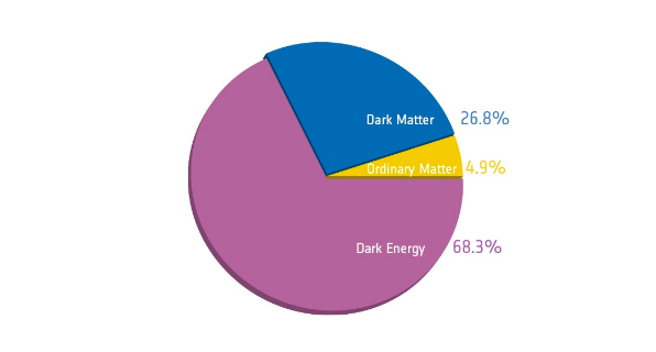
${\mathrm{\Omega }}_{\mathrm{\Lambda }}=0.68$ (5.22)

Which completes the cosmological pie in fig. 9.

This substance then rules the present evolution of the universe yet cosmology is the only evidence we have for it. If we go back to the action in eq. 4.5 we find that ${\rho }_{\mathrm{\Lambda }}$ as defined in the ratio $\mathrm{\Omega }$ appears as a constant in the action; ${\rho }_{\mathrm{\Lambda }}$ is the energy density when there is nothing else: the energy density of the vacuum. It is in a sense such an elementary term yet in most applications we do not see this energy density; we are interested in differences in energy. We study the kinetic energies of particles or differences in potential energies when we change their separation. Gravity however, through, Einstein field equations, is sensitive to the total energy density including that of empty space.

The description of this energy density as a substance in the stress energy tensor can be made in full by defining

$T_{\mathrm{\Lambda }}^{\mu \nu }\equiv$ ${\rho }_{\mathrm{\Lambda }}{g}^{\mu \nu }={\displaystyle \frac{\mathrm{\Lambda }}{8\pi G_N}}{g}^{\mu \nu }$ $\rho =$ ${\displaystyle \frac{\mathrm{\Lambda }}{8\pi G_N}}\mathit{\hspace{1em}\hspace{1em}}𝒫=-{\displaystyle \frac{\mathrm{\Lambda }}{8\pi G_N}}$ (5.23)

Unlike other contributions this density is independent of $a(t)$ which means a constant Hubble rate. This in turn has the rather dramatic effect of an accelerated expansion, if we resort back to the second Friedman equation

$2{\displaystyle \frac{\ddot{a}}{a}}$ $=-8\pi G_N\left(𝒫+{\displaystyle \frac{\rho }{3}}\right)$ (5.24)

where we used the first equation to substitute $H^2$. One has therefore that all positive or zero pressure substances produce a deceleration in the expansion. A cosmological constant however with a negative pressure as in eq. (5.23) overcomes the $\rho$ contribution for an accelerated expansion instead. To recall what negative pressure means, a refresher of thermodynamics where the change in internal energy (extensive magnitude) is, for change in volume

$dE=-𝒫dV$ (5.25)

So internal energy (again extensive quantity) increases with volume.

As a last word to spice up the discussion and give a sense of how little we know on the subject, we can take our theory of Nature today, the pinnacle of human knowledge that is the Standard Model and try to estimate $\mathrm{\Lambda }$. A prediction strictly speaking is not possible since we take the action to be our definition of the model so $\mathrm{\Lambda }$ is an input not an output; we can however estimate the quantum corrections on top of this input that give the effective $\mathrm{\Lambda }$. In an exercise in dimensional analysis and $4\pi$ counting which you should be familiar with by the end of the MSc one can estimate

$\delta \left({\displaystyle \frac{\mathrm{\Lambda }}{8\pi G_N}}\right)\sim {\displaystyle \frac{m_H^4}{16{\pi }^2}}$ (5.26)

You can amuse yourself to see how off is this estimate, given that $m_H$ is the Higgs mass $125$GeV and $\mathrm{\Lambda }\simeq 4.3\times {10}^{-66}$eV${}^2$

Problems

I (i) Given the average energy of a photon, proton and $T_0$, $m_p\sim 1$GeV use the value of the critical density and the contribution on the pie chart to estimate how many photons and protons are there on average per cm${}^3$, (ii) Neutrinos have a temperature a factor $0.7$ below that of the photons and their abundance is given by $0.18T_{\nu }^3$ estimate their abundance, (iii) Assume dark matter is made of a single species of non-relativistic particles with mass $m_{\mathrm{dm}}$ and derive an expression for the abundance of dark matter $n_{\chi }$ as a function of the mass.
II Derive yourself the bound on the universe radius starting from eq.  and using the critical density.
III Compute the luminosity distance for two z’s, start from recasting Friedman equation into the dependence of Hubble on redshift $H(z)$ for a matter dominated and CC dominated universe. Work out the integral for a matter dominated and cosmological constant dominated universes (both flat) to obtain

$d_L$ $={\displaystyle \frac{1+z}{H_0}}2\left(1-{\displaystyle \frac{1}{\sqrt{1+z}}}\right)\mathit{\hspace{1em}}{\mathrm{\Omega }}_m=1$ $d_L$ $={\displaystyle \frac{1+z}{H_0}}z\mathit{\hspace{1em}}{\mathrm{\Omega }}_{\mathrm{\Lambda }}=1$ (5.27)

Plot these two lines and the experimental points for 1992P and 1997ap. Which line falls closer?

6 The universe in equilibrium

Electromagnetic radiation in the present composition of the universe is a tiny part of the total yet it holds the key to the early epoch of our universe. The reason for this is twofold, $i)$ this radiation is what remains of the primordial plasma in an almost frozen-in-time form and $ii)$ due to the scaling with $a(t)$ of radiation energy density, this used to be the dominant component in Friedmann equation at early times and ruled the expansion.

6.1 Equilibrium distribution

As outlined in the introduction, studying the CMB is studing a substance in equilibrium, so first for completeness we go through an overview of statistical mechanics (we momentarily restore $\mathrm{\hslash }$ in our equations to remind us of the quantum nature). Consider phase space ($\underset{¯}{x},\underset{¯}{p}$) for a particle species with energy $E$ given to a good approximation by that of a free particle $E^2=m^2+p^2$. Heisenberg’s uncertainty principle states that the tighter one can ‘pack’ a particle in phase space is to have it inside $\mathrm{\Delta }{x}^3\mathrm{\Delta }{p}^3={(2\pi \mathrm{\hslash })}^3$. This is the unit of phase-space volume to count particles which is to say

$Vn={\displaystyle \int \frac{d^{3}x{d}^{3}p}{{(2\pi \mathrm{\hslash })}^3}f(x,p)}$ (6.1)

with $f(x,p)$ a probability distribution in phase space and $V$, $n$ the volume and particle abundance. Alternatively, if you find this argument too vague, you can put particles on a box of length $L$ to find the density of states through the quantization of momentum:

$p^i$ $={\displaystyle \frac{2\pi \mathrm{\hslash }}{L}}{k}^i$ $d(\mathrm{States})={(dk)}^3={\displaystyle \frac{L^3}{{(2\pi \mathrm{\hslash })}^3}}{(dp)}^3={\displaystyle \frac{d^{3}x{d}^{3}p}{{(2\pi )}^3}}$ (6.2)

with $k^i$ a 3-vector with positive integer values, $k^{1,2,3}=(0,1,2,\mathrm{\dots })$.

Next one has that in a thermal distribution the number of particles is not conserved and we consider placing any number of particles in any of the states in phase space. Obviously the options are different whether one has a fermion or a boson so the two are discussed in parallel for Bose-Einstein (BE) or Pauli-Dirac (PD) distributions respectively. Consider first the partition function at fixed energy $E$; for a boson we can have any number of particles in a given state, call it $N$, and so the energy is $N\times E$. The partition function is then

$Z{(E)}_{\mathrm{BE}}={\displaystyle \sum _N}{e}^{-N(E-\mu )/T}={\displaystyle \frac{1}{1-e^{-(E-\mu )/T}}}$ (6.3)

where we also included a chemical potential $\mu$ for completeness and we used the geometric series expansion to sum the series. The sum for fermions is much simpler, one or none

$Z{(E)}_{\mathrm{PD}}=1+e^{-(E-\mu )/(T{k}_B)}$ (6.4)

In the following we will set Boltzmann constant

$k_B=8.617\times {10}^{-5}{\text{eV K}}^{-1}$ (6.5)

to $1$, implying temperature and energy have the same units. Then the expected number of particles per phase space for a given energy E reads like the number of particles $N$ times the respective probability $e^{-NE}$ over the sum of probabilities $Z$. This can be synthesized in the derivative:

(6.6)

This completes all components we need to describe the thermal ensemble of particles and one can put it to use right away in the CMB today. Experimental evidence indicates that the chemical potential can be neglected for the CMB and indeed this will be the case for substances in chemical equilibrium as we shall see in chapter 8. The number density of photons in the bath is then

$n_{\gamma }=g_{\gamma }{\displaystyle \int \frac{d{p}^3}{{(2\pi )}^3}\frac{1}{e^{E/T}-1}}=g_{\gamma }{\displaystyle \frac{4\pi }{{(2\pi )}^3}}{T}^3{\displaystyle \int \frac{y^{2}dy}{e^y-1}}={\displaystyle \frac{g_{\gamma }}{{\pi }^2}}\zeta (3)T^3$ (6.7)

where the degeneracy factor $g_{\gamma }=2$ comes from the 2 possible polarizations of photons, we changed variables to $y=p/T$ and $\xi$ is Riemann zeta function with $\xi (3)\simeq 1.202$. The energy per unit volume in the CMB is on the other hand the integral over the distribution function times the energy

${\rho }_{\gamma }=g_{\gamma }{\displaystyle \int \frac{d^{3}p}{{(2\pi )}^3}E(p)f_{\mathrm{BE}}(x,p)}=g_{\gamma }{\displaystyle \frac{(4\pi )T^4}{{(2\pi )}^3}}{\displaystyle {\int }_0^{\mathrm{\infty }}}𝑑y{\displaystyle \frac{y^3}{e^y-1}}=g_{\gamma }{\displaystyle \frac{{\pi }^2}{30}}{T}^4$ (6.8)

where in this case Riemann’s zeta function has an exact expression which we substituted in, $\zeta (4)={\pi }^4/90$. We have therefore now computed the proportionality constant that we took as a given in chapter 5, eq. 5.7.

The difference in the case of relativistic fermions is slight but computable exactly

${\rho }_{\nu }=g_{\nu }{\displaystyle \int \frac{d^{3}p}{{(2\pi )}^3}E(p)f_{\mathrm{PD}}(x,p)}=g_{\nu }{\displaystyle \frac{(4\pi )T^4}{{(2\pi )}^3}}{\displaystyle {\int }_0^{\mathrm{\infty }}}𝑑z{\displaystyle \frac{z^3}{e^z+1}}={\displaystyle \frac{7}{8}}{g}_{\nu }{\displaystyle \frac{{\pi }^2}{30}}{T}^4$ (6.9)

where we took a neutrino to be our massless fermion and in the Standard Model $g_{\nu }=2$ for the two spins states. In reality there are three neutrinos and they are massive, whose consequences we will see on due time.

One can put the two cases together in an expression for relativistic particles as:

$${\rho }_{\mathrm{rad}}=g_{\star }\frac{{\pi }^2}{30}{T}^4$$ $g_{\star }$ $=\left({\displaystyle \sum \mathrm{boson}\mathrm{species}}\right)+{\displaystyle \frac{7}{8}}\left({\displaystyle \sum \mathrm{fermion}\mathrm{species}}\right)$ (6.10)

assuming all particles have the same temperature $T$. If some species have a different temperature one can still use the above definition with a reference temperature and the degeneracy $g_{\star }$ of some species rescaled by ${(T/T^{\prime })}^4$.

Another quantity we will find useful is the entropy density for a particle with negligible chemical potential which is defined as

$s={\displaystyle \frac{\rho +𝒫}{T}}={\displaystyle \int \frac{d{p}^3}{{(2\pi )}^3}f(p,x)\left(\frac{E}{T}+\frac{p^2}{3ET}\right)}$ (6.11)

recalling thermodynamics relation $TS=V\rho +V𝒫$. For all relevant processes of study here the entropy will be dominated by relativistic particles in which case $Ts=4\rho /3$.

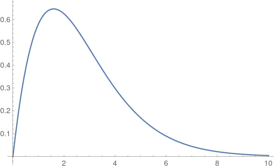
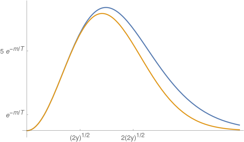
Let us turn now to the other type of contributions in Friedmann’s equation. For a non-relativistic particle the distribution function can be approximated as:

$f(E)={\displaystyle \frac{1}{e^{\sqrt{m^2+p^2}/T}\mp 1}}\stackrel{p,T\ll m}{\simeq }{\displaystyle \frac{1}{e^{m/T+p^2/(2mT)}}}$ (6.12)

Where we see that in this approximation the distribution is independent of the bosonic or fermionic nature. The approximation is off for the high energy tail $p^2\gg mT$ where the distribution falls as an exponential $e^{-p/T}$ and not a Gaussian as the approximation above gives; this can be appreciated in fig. 10. Nonetheless for integrated magnitudes this part of the spectrum contributes a exponentially small share and we can approximate for non relativistic ($m\gg T$), $\mu =0$, particles in the plasma:

$n_{\mathrm{N}.\mathrm{R}.}=g{\displaystyle \frac{4\pi }{{(2\pi )}^2}}{e}^{-m/T}{(mT)}^{3/2}{\displaystyle {\int }_0^{\mathrm{\infty }}}{y}^2{e}^{-y^2/2}𝑑y=g{e}^{-m/T}{\left({\displaystyle \frac{mT}{2\pi }}\right)}^{3/2}$ (6.13)

Equivalently any other magnitude will have an exponential suppression $e^{-m/T}$ and units $\sqrt{mT}$. We can understand the exponentially small number of particles in simple terms, the average energy $T$ available for interactions is not enough to produce the species of mass $m$, only those particles in the high $p$ tail of the distribution have enough energy but their abundance is smaller by precisely this exponential factor.

Figure 10: Black body spectrum for particle density as a function of $x=p/T$ for $m=0$ LHS and $m/T=10$ with the approximation of eq. in yellow.

6.2 Equilibrium in an expanding universe

This far the discussion has overlooked the fact that this thermal bath is placed in an expanding universe. What keeps the bath in equilibrium is the continuous interaction of particles with one another; if the expansion rate is slower than this interaction rate of the particles the equilibrium distribution is preserved. The two magnitudes to compare are therefore the i) Hubble rate $H(t)$ whose inverse gives the time it takes for the universe to double in size versus ii) the interaction rate $\mathrm{\Gamma }$ whose inverse gives the average time between interactions. This number can be estimated as $\sigma vn$ with $\sigma$ the cross section, $v$ the relative velocity and $n$ the number density of particles that the species we are interested in interacts with.

For now let us assume $\mathrm{\Gamma }\gg H$ so equilibrium is preserved. The adiabatic approximation then applies which in practice means the expressions we were using are valid but now the magnitudes change with time $t$.

Let us connect first the expression for the time evolution of radiation energy derived in the first chapters with that obtained here for a distribution in equilibrium:

${\rho }_{\gamma }(t)={\displaystyle \frac{a{(t_i)}^4}{a{(t)}^4}}\rho (t_i)=g{\displaystyle \frac{{\pi }^2}{30}}{T}^4$ (6.14)

which is consistent if the temperature scales as

$T(t)={\displaystyle \frac{a(t_i)}{a(t)}}T(t_i)$ (6.15)

That is, the plasma cools as time passes and space expands; when the universe doubles in size the temperature falls by a half.

The same matching does not apply to non-relativistic particles however; eq. (6.13) scales with $T^{3/2}$ which given the above would imply $n\sim a^{-3/2}$ yet we know for matter $n\sim a^{-3}$. The answer to this apparent contradiction is many-fold and we should unfold it in subsequent chapters. The short explanation is that we cannot neglect the chemical potential for matter which today is very far from an equilibrium.

The abundance in eq. (6.13) today can be understood as produced by photons so high up in energy in the tail of the distribution that they can pair produce non-relativistic particles, say baryons. These type of photons are however so rare that the abundance of these thermal baryons is negligible for all purposes, $n_p^{eq}/n_{\gamma }\sim e^{-m/T_0}\sim {10}^{-{10}^{12}}$.

Finally as pointed out in the beginning the fact that the energy density in radiation scales with the most inverse powers of the scale factor means in return that this type of energy used to dominate the total budget of the universe. The Friedman equation then reads in this regime

${\displaystyle \frac{{\dot{a}}^2}{a^2}}$ $={\displaystyle \frac{8\pi G_N}{3}}{g}_{\star }{\displaystyle \frac{{\pi }^2}{30}}{T}^4$ $z$ $\gg {10}^4$ (6.16)

where $g_{\star }$ counts the number of relativistic degrees of freedom as in eq. (6.10).

6.3 Entropy conservation

One useful conservation equation is that of entropy for relativistic particles. One can derive this from the divergence of the stress energy tensor ${\nabla }_{\mu }{T}_{\nu }^{\mu }$ being vanishing, in particular for the first component we have, from eq. (4.17)

${\nabla }_{\mu }{T}_{\mathrm{\hspace{0.17em}\hspace{0.17em}0}}^{\mu }={\displaystyle \frac{\partial \rho }{\partial t}}+{\displaystyle \frac{\dot{a}}{a}}(3\rho +3𝒫)={\displaystyle \frac{\partial }{a^3\partial t}}{a}^3(\rho +𝒫)-{\displaystyle \frac{\partial 𝒫}{\partial t}}=0$ (6.17)

Using either Bose Einstein or Fermi-Dirac distributions with a dependence solely on the energy one can derive for relativistic particles;

${\displaystyle \frac{\partial 𝒫}{\partial T}}={\displaystyle \frac{\partial }{\partial T}}{\displaystyle \int \frac{d^{3}p}{{(2\pi )}^3}\frac{p^2}{3E(p)}f(E/T)}\stackrel{m\ll T}{=}{\displaystyle \int \frac{d^{3}p}{{(2\pi )}^3}\frac{p}{3}\left(-\frac{p}{T}\right)\frac{\partial }{\partial p}f(p/T)}$ (6.18)

next integration by parts where the boundary term vanishes gives the relation $\partial 𝒫/\partial T=(\rho +𝒫)/T$ which back in the conservation equation

${\displaystyle \frac{1}{T}}{\nabla }_{\mu }{T}_{\mathrm{\hspace{0.17em}\hspace{0.17em}0}}^{\mu }={\displaystyle \frac{1}{T}}{\displaystyle \frac{\partial }{a^3\partial t}}{a}^3(\rho +𝒫)-{\displaystyle \frac{dT}{dt}}{\displaystyle \frac{\rho +𝒫}{T^2}}={\displaystyle \frac{\partial }{a^3\partial t}}{\displaystyle \frac{a^3(\rho +𝒫)}{T}}={\displaystyle \frac{1}{a^3}}\boxed{{\displaystyle \frac{\partial (a^{3}s)}{\partial t}}=0}$ (6.19)

with says the time dependence of entropy density $s=(\rho +𝒫)/T$ is given by the factor $a^{-3}(t)$. You might be familiar with the conservation law $\nabla T$, which comes from the action invariance under space-time shifts, giving in other settings total energy-momentum conservation, like in say QFT in Minkowski space; here however the situation is more aptly described by fluid mechanics and thermodynamics given that radiation’s pressure means the substance does work with the expansion and it is entropy instead that is conserved.

Problems

I Now that we have the distributions for relativistic spin 1 and 1/2 particles compute the exact expression for the abundance of photons and neutrinos given $T_{\nu }=$ (recall there’s 3 $\nu$ in the SM with one chirality only.) [Hint: $n_{PD}=3n_{BE}/4$]
II Check the result in eq. 6.6 explicitly using the expressions for $Z_{BE}$, $Z_{PD}$.
III At temperatures above the MeV photons, neutrinos electrons and positrons are present in the plasma with the same temperature, what is $g_{\star }$ then? At the EW scale $246$GeV all particles in the SM can be taken relativitic, what would $g_{\star }$ be then?
IV Show that Pauli-Dirac and Bose-Einstein distributions are related as $n_{\mathrm{PD}}=3/4n_{\mathrm{BE}}$ ${\rho }_{\mathrm{PD}}=7/8{\rho }_{\mathrm{BE}}$ as part of the series of averages of powers of energy

${\displaystyle \int \frac{d^{3}p}{{(2\pi )}^3}\frac{p^n}{e^{p/T}+1}}=\left(1-{\displaystyle \frac{1}{2^{n+2}}}\right){\displaystyle \int \frac{d^{3}p}{{(2\pi )}^3}\frac{p^n}{e^{p/T}-1}}$ (6.20)

[Hint: Use $f_{\mathrm{BE}}(E)-f_{\mathrm{PD}}(E)=2f_{\mathrm{BE}}(2E)$ and a change of variables, you do not have to perform the integrals explicitly]

7 Turning back time

The framework has now been laid for the study of the universe at its largest scale. The observations that determine the state of the cosmos today together with the evolution equations in the form of Friedman’s equations allow to turn back the dial of time and reconstruct the history of the universe. The next chapters will take us back in time as far as solid evidence can take us.

Reviewing the components of the universe we found that the main contribution is in the form of a cosmological constant followed by matter contribution (both of them being none of the substances we can produce in a lab), we can take the short term evolution of the universe then given by

${\left({\displaystyle \frac{1}{a}}{\displaystyle \frac{da}{dt}}\right)}^2=H_0^2\left({\mathrm{\Omega }}_{\mathrm{\Lambda }}+{\displaystyle \frac{{\mathrm{\Omega }}_m}{a{(t)}^3}}\right)$ (7.1)

with the definition of $\mathrm{\Omega }$ and critical density as in (5.4). One can solve this differential equation exactly to find the growth of the universe in the future, but also how the growth used to be. Although the exact solution can be found with a little work and a table integral, the two limiting behaviours are good approximations in the respective regimes

${\left({\displaystyle \frac{1}{a}}{\displaystyle \frac{da}{dt}}\right)}^2$ $=H_0^2{\displaystyle \frac{{\mathrm{\Omega }}_m}{a{(t)}^3}}\mathit{\hspace{1em}\hspace{1em}}t\ll H_0^{-1};$ ${\left({\displaystyle \frac{1}{a}}{\displaystyle \frac{da}{dt}}\right)}^2$ $=H_0^2{\mathrm{\Omega }}_{\mathrm{\Lambda }}\mathit{\hspace{1em}\hspace{1em}}{H}_0\gg t_0$ (7.2)

The one thing left to specify for the explicit solutions are the original conditions, which are taken as

$a(0)$ $=0$ (7.3)

given that we define the origin of time as the singular point. The solutions in the two regimes then are simple to find

$a(t)$ $={\left({\displaystyle \frac{3}{2}}\sqrt{{\mathrm{\Omega }}_m}{H}_{0}t\right)}^{2/3},t\ll H_0;$ $a(t)=a(t_{+})e^{H_0\sqrt{{\mathrm{\Omega }}_{\mathrm{\Lambda }}}(t-t_{+})},t\gg H_0^{-1}.$ (7.4)

Figure 11: Time dependence of the scale factor for a matter and cosmological constant dominated universe

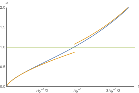
where $t_{+}$ is reference time in the future. The initial conditions are imposed in early times so that the solution in that regime is fully specified. For the late time region the constants in the solution as given depend on an integral which covers the full range $t=0,t_{+}\gg H_0^{-1}$. This piece of information we borrow from the exact solution to find

$a(t)={\left[{\displaystyle \frac{{\mathrm{\Omega }}_m}{4{\mathrm{\Omega }}_{\mathrm{\Lambda }}}}\right]}^{1/3}{e}^{H_0\sqrt{{\mathrm{\Omega }}_{\mathrm{\Lambda }}}t},t\gg H_0^{-1}.$ (7.5)

The plot in fig. 11 shows the shape of the exact solution and approximations. As can be seen just one half of the Hubble time into either the future or the past puts us in a regime in which the matter only or $\mathrm{\Lambda }$ only solution is an excellent one.

Given our present knowledge the fate of the universe is to fall into an accelerated expansion with an exponential growth. This statement must however be put in context, first the daily remainder that the scales we talk about here are cosmological, so for example our galaxy and Andromeda will not be pulled apart not to mention our galaxy itself. This is because the gravitational field that bounds us together is much stronger than the Hubble drag. Second, as the solution shows we enter a fully accelerated phase in half the Hubble time, 7000 million years from now; making extrapolations so far in time might well be an overreach. That being said the information we have today points to this acceleration taking over till the end of time.

7.1 The epochs of the universe

Next lets turn our gaze back. First observe that present time is derived from the solution rather than put in. One has $a(t_0)=1$ which, given we solution $a(t)$ with $a(0)=0$, turns into an equation that one solves for to find $t_0$. The exact solution then yields a value for $t_0$ given by the point where the horizontal and blue line cross. This returns

$t_0=0.949H_0^{-1}={\displaystyle \frac{0.949}{100h}}{\text{km }}^{-1}\text{ s Mpc}=13.9\times {10}^9\mathrm{years}$ (7.6)

You can derive this expression for the age of the universe yourself following the problems at the end of this chapter.

Again from fig. 11 one infers that before the half life of the universe one can neglect the cosmological constant contribution which corresponds to since at this time

${\displaystyle \frac{{\mathrm{\Omega }}_m}{a^3(t_0/2)}}$ $\simeq 8{\mathrm{\Omega }}_m\simeq 2.4$ $\mathrm{vs}$ ${\mathrm{\Omega }}_{\mathrm{\Lambda }}$ $\simeq 0.7$ (7.7)

This follows from the fact that matter density dilutes with $a^3$ and it used to be much larger in the past. For that purpose radiation dilutes even faster with $a^4$ so it must have been even more relevant in early times.

Indeed we can estimate at what scale factor matter and radiation energy densities where around the same

${\displaystyle \frac{{\mathrm{\Omega }}_m}{a{(t)}^3}}={(z+1)}^3{\mathrm{\Omega }}_m={\displaystyle \frac{{\mathrm{\Omega }}_r}{a{(t)}^4}}={(1+z)}^4{\mathrm{\Omega }}_r$ (7.8)

Which returns $z_{eq}\simeq 3.4\times {10}^3$ with this event in time known as matter-radiation equality or sometimes just equality. The universe was $3400$ times smaller which corresponds to about a hundred thousand years old. Befor this time therefore radiation dictated the expansion of the universe in the form of the CMB photons and neutrinos. The CMB had a temperature then of:

$T(t_{eq})=(z_{eq}+1)T_0=0.80\mathrm{eV}$ (7.9)

The Hubble rate and growth of the universe then was determined by the energy in radiation which we can express in terms of the temperature as given in eq. (6.16):

$$H{(t)}^2=\frac{8\pi G_N}{3}\frac{g_{\star }{\pi }^2}{30}{T}^4$$ (7.10)

where $g_{\star }$ counts the effective degrees of freedom.

At such early times $t$ the universe looked very different; matter had not begun to condense and collapse into galaxies due to gravity since the interaction with photons was so frequent and energetic that kept it in thermal equilibrium at the same temperature. Earlier still at temperatures of $T\sim 2m_e$ the average energy of photons was high enough that pairs of electron and positrons were produced with abundances given by the Pauli-Dirac distributions of chapter 6. This also means that the number of relativistic degrees of freedom $g_{\star }$ used to be different. Earlier still at higher temperatures other known particles would be produced as mass thresholds are crossed, as to which ones one can get this information from particle physics.

This gives you an idea of why particle physics and cosmology are connected fields. The primordial plasma is a ‘particle physics’ experiment where the evolution and properties of the plasma can be traced with simple mathematics to fundamental physics. Further still, evolution in cosmology is ruled by gravity and offers an experimentally testable set-up to look into an interaction which in conventional particle physics experiments is far too weak to be relevant.

Case in point, $g_{\star }$ for $T=1eV$ one should be able to infer from particle physics by looking at how many species are there lighter than that value. Photons in the CMB with two polarizations and $g_{\gamma }=2$ of course but a look at particle listings reminds us there are also neutrinos with an upper bound on their masses of precisely about eV. We know there are 3 species of neutrinos ${\nu }_e,{\nu }_{\mu },{\nu }_{\tau }$ each with two spin states $g_{\nu }=3\times 2$. Nevertheless do they have the same temperature as the CMB?

The answer is no, they are not in thermal equilibrium with the photons and do not share the same temperature, they are actually cooler.

Neutrinos are very weakly interacting particles and they fell out of touch with the plasma at temperatures $T\sim$MeV scale, as to why this value we will find out in the next chapter. At that temperature the plasma included electrons and positrons ($m_e\sim 0.5$MeV) yet they were on their way out as when temperature dipped below MeV they annihilated into photons $e^{+}{e}^{-}\to \gamma \gamma$. This process heated the plasma and we will estimate by how much using entropy conservation.

At times $t_{-}$ when the temperature was above $m_e$ and $e^{+}{e}^{-}$ where abundant but neutrinos had already decoupled the entropy on the plasma was

$s(t_{-})={\displaystyle \frac{2{\pi }^2}{45}}{g}_{\star }^{\mathrm{bath}}(t_{-})T^3(t_{-})={\displaystyle \frac{2{\pi }^2}{45}}\left(g_{\gamma }+{\displaystyle \frac{7}{8}}{g}_{e^{+}}+{\displaystyle \frac{7}{8}}{g}_{e^{-}}\right)T^3(t_{-})$ (7.11)

whereas after the annihilation the entropy would read

$s(t_{+})$ $={\displaystyle \frac{2{\pi }^2}{45}}{g}_{\gamma }{T}_{\gamma }^3$ (7.12)

where we called $T_{\gamma }=T(t_{+})$ the temperature of photons in the CMB after $e^{+}{e}^{-}$ annihilation. Entropy conservation tells us $s{a}^3$ is conserved and so

${(a(t_{-})T(t_{-}))}^3{g}_{\star }(t_{-})=g_{\gamma }{(a(t_{+})T_{\gamma })}^3$ (7.13)

In the meantime neutrinos were decoupled watching things unfold from the sideline; this means their distribution was Pauli-Dirac with a temperature $T_{\nu }$ even if they were non-interacting, much like the CMB today. This neutrino temperature simply scales with the expansion oblivious to what is going on in the bath. Furthermore at early times $t_{-}$ this temperature was the same as that of the bath so

$T_{\nu }(t)={\displaystyle \frac{a(t_{-})T(t_{-})}{a(t)}}$ (7.14)

so one can rewrite eq. (7.13) to read

${\displaystyle \frac{T_{\nu }^3(t_{+})}{T_{\gamma }^3(t_{+})}}={\displaystyle \frac{g_{\gamma }}{g_{\star }^{\mathrm{bath}}(t_{-})}}={\displaystyle \frac{4}{11}}$ (7.15)

which means neutrinos are a factor ${(4/11)}^{1/3}\sim 0.7$ cooler than photons today.

Therefore after $T\sim$ MeV ($e^{+}{e}^{-}$ annihilation) and before $T\sim$ eV (when neutrinos turn non-relativistic) the energy density on radiation is

${\rho }_r={\displaystyle \frac{{\pi }^2}{30}}{g}_{\gamma }{T}_{\gamma }^4+{\displaystyle \frac{{\pi }^2}{30}}{g}_{\nu }{\displaystyle \frac{7}{8}}{T}_{\nu }^4={\rho }_{\gamma }\left(1+{\displaystyle \frac{7}{8}}{\left({\displaystyle \frac{4}{11}}\right)}^{4/3}{N}_{\mathrm{eff}}\right)$ (7.16)

with $N_{\mathrm{eff}}=3$ for the 3 neutrino species. We went to the trouble of introducing $N_{\mathrm{eff}}$ because in general there might be other relativistic species contributing to the total which would manifest in $N_{\mathrm{eff}}\ne 3$ and this variable is a commonplace observable defined to reflect this possibility; at present cosmological data sets $N_{\mathrm{eff}}=2.99\pm 0.34$ [2].

7.2 Interchangeable labels for history

The labels to refer to events in the universe’s history have been piling up: time $t$, conformal time $\eta$, scale factor $a$, redshift $z$, and now temperature $T$. All of them either increase or decrease monotonically and so any two of them are univocally connected by a mapping, which might involve solving an ODE or a given algebraic relation. Yet if after all they are interchangeable labels why don’t we stick to one and write everything else in terms of our chosen variable?

The answer is that depending on the event and epoch one is looking at one of these variables will be specially suited to describe the physics. It is therefore good to know how to change variables (labels) and what is the use of each one, so here is a rough guide

• Time $t$ is the time as inertial observers would measure it and for the radiation and matter dominated eras, its inverse gives an order of magnitude estimate of Hubble $H\sim t^{-1}$.

• Conformal time is the time coordinate for a transformed metric as in eq. 3.25 in conformal form. It is useful for discussing causality and as we shall see evolution of perturbations.

• Scale factor $a(t)$ tracks the size of our universe and given the present pie-chart breakdown of energy density is a useful marker for the different eras of the universe: radiation/matter/CC dominated.

• Redshift $z$ is related to the scale factor algebraically $1+z=1/a$ so for early enough times is simply its inverse yet it is also easy to extract experimentally observing standardized luminous objects.

• Temperature $T$ which unless otherwise stated refers to photon temperature, signals which species are in thermal equilibrium and scales, away from mass thresholds, with the inverse of the scale factor.

(a) Relativistic degrees of freedoms in the plasma

(b) Our labels for the history of the universe

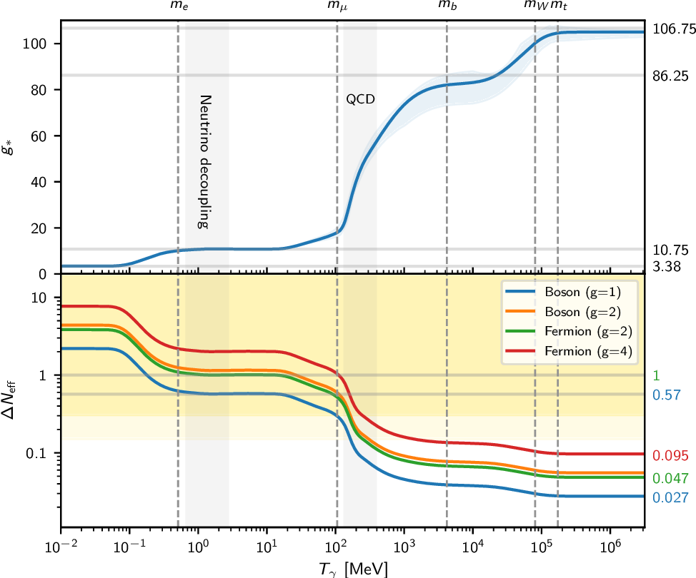
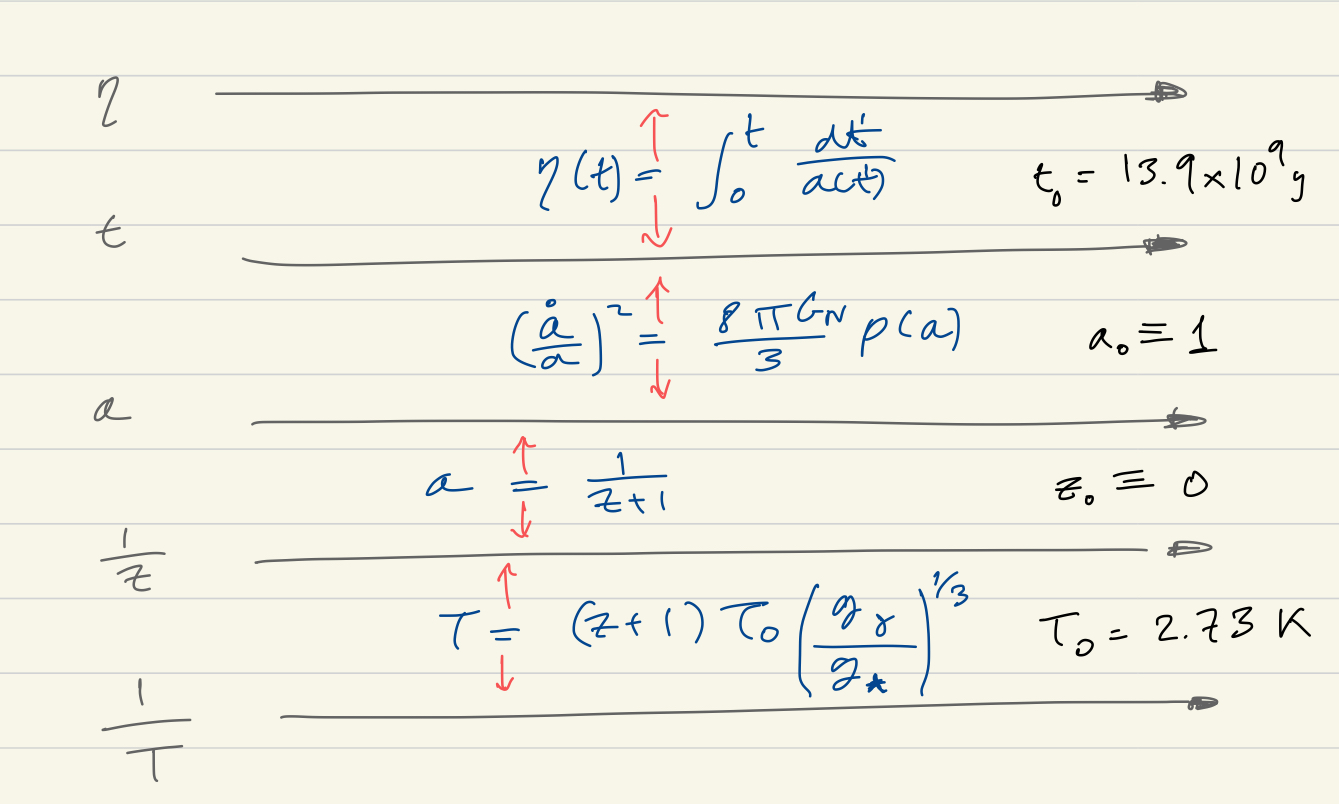
Problems

I Consider a radiation dominated universe ${\mathrm{\Omega }}_r\simeq 1$ in Friedman’s equation and with the initial conditions $a(0)=0$ compute $a(t)$, $z(t)$, $\eta (t)$, $H(t)$. Assuming radiation follows a black body distribution with temperature $T$ and $g_{\star }$ degrees of freedom compute $T(t)$. Which of these variables do and don’t depend on $H_0$?
II Determine the redshift of equality substituting in eq. 7.8 the energy density of the CMB 5.8. Do you get the same result $z_{eq}=3.400$? What is the temperature at that redshift and what is wrong with the calculation? Use eq. (7.16) to compute $z_{eq}$ instead.
III Let’s solve exactly eq. (7.1) with $a(0)=0$ and find the age of the universe and the normalization of the asymptotic limits. You can do it in your favourite way but here’s a hint

${\displaystyle \frac{d}{dx}}\text{ArcTanh}\left({\displaystyle \frac{1}{\sqrt{1+L(x)}}}\right)=-{\displaystyle \frac{1}{2}}{\displaystyle \frac{1}{\sqrt{1+L(x)}}}{\displaystyle \frac{d\log (L(x))}{dx}}$ (7.17)

with ArcTanh the inverse hyperbolic tangent ArcTanh$(x)=1/2\log ((1+x)/(1-x))$. Use the values of $\mathrm{\Omega }$ from chapter to find $0.949$.

8 Boltzmann Equations

The primordial plasma back when the temperature was around MeV contained photons, $e^{+}$, $e^{-}$ and neutrinos in chemical equilibrium ($\mu =0$) distributions. As we shall see it also contained the baryons that formed the known universe in thermal but not chemical equilibrium ($\mu \ne 0$). How does one determine what particles were in equilibrium in the original soup and for how long? Looking into this question will lead into another, more ambitious one; what aspects of the universe can one account for from the fundamental properties of particles and the evolution of the original plasma?

Figure 12: Particles $i,j$ $\to$ particles $k,j$ reaction

The answer lies in Boltzmann equations, applied to our homogeneous and isotropic approximation to the universe. Let us compute the change with time in the number of particles of a given species $i$. First, the change in particle abundance of the species $i$ we are already familiar with is the decrease with the expansion of the universe. One can make this explicit with the current $J_{\mu }^i=(n_i,\underset{¯}{0})$ conservation equation

${\nabla }_{\mu }{J}^{\mu }={\displaystyle \frac{\partial n_i}{\partial t}}+{\mathrm{\Gamma }}_{k0}^k{n}_i={\displaystyle \frac{\partial n_i}{\partial t}}+3{\displaystyle \frac{a^{\prime }}{a}}{n}_i$ (8.1)

This will equal 0 in the absence of interactions with the solution $n_i\propto a^{-3}$ that presents the volume dilution with expansion as intuition suggests. If the number of $i$ particles is not a conserved number in the presence of interactions, that is at the fundamental level, there will be a source term. Consider first a process in the soup with 2 different species of particles $i,j$ coming in and 2 other $k,l$ coming out. The process has an amplitude $ℳ$ which one can compute in quantum field theory given the interaction Lagrangian but here we take it as a given. This process we assume is the leading reaction which depletes the number of $i$ particles. However the inverse reaction $k,l$ to $i,j$ must also be possible and this will increase the number of $i$ particles. One has then the two competing reactions, each possible for any momenta $p_i,p_j,p_k,p_l$ such that the total is conserved so we integrate over momentum space as

${\displaystyle \frac{1}{a^3}}{\displaystyle \frac{d{a}^3{n}_i}{dt}}=$ ${\displaystyle \int \frac{d{p}_i^3}{{(2\pi )}^{3}2E_i}\frac{d{p}_j^3}{{(2\pi )}^{3}2E_j}\frac{d{p}_k^3}{{(2\pi )}^{3}2E_k}\frac{d{p}_l^3}{{(2\pi )}^{3}2E_l}{(2\pi )}^4{\delta }^4(p_i+p_j-p_k-p_l)}$

$\times {|ℳ|}^2(f_k{f}_l(1\pm f_i)(1\pm f_j)-f_i{f}_j(1\pm f_k)(1\pm f_l))$ (8.2)

The LHS above is a rewriting of eq. (8.1) whereas the collision term on the RHS has the integral over Lorentz invariant phase space which you might already be familiar with from QFT. In addition now there are factors of the distributions $f$; the second term in the second line is proportional to $f_i$ and $f_j$ since they are the abundances of the initial states in $i,j\to k,l$ whereas the extra ($1\pm f_k$) terms arise from Pauli blocking (-) when the particle $k$ is a fermion and the state might be occupied already or Bose enhancement (+) for a boson. The first term is the inverse reaction and the relative sign comes from one reaction increasing and the other decreasing the number of $i$ particles. Finally we assumed $ℳ$ is the same for the inverse and direct process which happens if CP (charge conjugation$\times$parity) symmetry is preserved.

This is Boltzmann’s equation for the abundance of particle species $i$. At face value is a formidable equation to formulate, let alone solve; it contains derivatives in time but integrals in momentum of the functions $f(t,p)$ we want to solve for and to obtain a closed system one needs the coupled equations for the other species distributions $f_j,f_k,f_l$. Luckily a number of approximations hold in the processes of interest which greatly simplify the system.

First, even when a particle abundance diverges from the equilibrium value, process which do not change the particle number (like Compton scattering) ensure a Bose-Einstein or Fermi-Dirac distribution is maintained, only with a time-dependent chemical potential $\mu (t)$. One can then substitute $f$ as a function of $\mu$, $E$ as given in chapter 6 and translate the differential equation into $\mu$. In addition, the relevant part of the distributions will be at $E-\mu$ above $T$, so the $\pm$ factors of bosonic or fermionic statistics can be neglected in favour of Boltzmann’s distribution.

All this makes the equation collapse into:

${\displaystyle \frac{1}{a^3}}{\displaystyle \frac{d{a}^3{n}_i}{dt}}=$ ${\displaystyle \int \frac{d{p}_i^3}{{(2\pi )}^{3}2E_i}\frac{d{p}_j^3}{{(2\pi )}^{3}2E_j}\frac{d{p}_k^3}{{(2\pi )}^{3}2E_k}\frac{d{p}_l^3}{{(2\pi )}^{3}2E_l}{(2\pi )}^4{\delta }^4(p_i+p_j-p_k-p_l)}$

$\times {|ℳ|}^2{e}^{-(E_i+E_j)/T}(e^{({\mu }_k+{\mu }_l)/T}-e^{({\mu }_i+{\mu }_j)/T})$ (8.3)

where we used energy conservation to factor out the exponential in initial energy. Next one can take the chemical potential exponentials out of the integrals and define the prefactor with use of the equilibrium, zero potential distribution:

$n_i^{(0)}\equiv$ ${\displaystyle \int \frac{d^3{p}_i}{{(2\pi )}^3}{e}^{-E_i/T}}$ (8.4)

$⟨\sigma v⟩\equiv$ ${\displaystyle \frac{1}{n_i^{(0)}{n}_j^{(0)}}}{\displaystyle \int \frac{d{p}_i^3}{{(2\pi )}^3}{e}^{-E_i/T}\frac{d{p}_j^3}{{(2\pi )}^3}{e}^{-E_j/T}\sigma v}$ (8.5)

$\sigma v=$ ${\displaystyle \int \frac{d{p}_k^3}{{(2\pi )}^{3}2E_k}\frac{d{p}_l^3}{{(2\pi )}^{3}2E_l}{(2\pi )}^4{\delta }^4(p_i+p_j-p_k-p_l)\frac{1}{4E_i{E}_j}{|ℳ|}^2}$ (8.6)

where the third line contains the definition of the cross section times velocity $\sigma v$ which you might be familiar with from QFT. The difference with the thermally averaged cross section times velocity $⟨\sigma v⟩$ being that there is a distribution of the initial states which one also integrates over; that being said the familiar cross section with centre of mass energy $E\sim T$ gives a good estimate for case of temperatures above particle masses. These definitions convert Boltzmann equation into

${\displaystyle \frac{1}{a^3}}{\displaystyle \frac{d{a}^3{n}_i}{dt}}=n_i^{(0)}{n}_j^{(0)}⟨\sigma v⟩\left({\displaystyle \frac{n_k{n}_l}{n_k^{(0)}{n}_l^{(0)}}}-{\displaystyle \frac{n_i{n}_j}{n_i^{(0)}{n}_j^{(0)}}}\right)$ (8.7)

where we used $n_i/n_i^{(0)}=e^{{\mu }_i/T}$. Although all we have done from eq. (8.3) to eq. (8.7) is to hide the integrals in definitions, these new magnitudes have physical meaning and are useful in discussing the behaviour and outcome of these equations for the dynamics.

The magnitude on the LHS has units of particle abundance per unit time and is of order $n_{i}H$ with $H$ the Hubble rate while on the RHS we have $n_i{n}_j\sigma v$. Whether the expansion or the reactions dominate will determine the evolution of a particle abundance so the dimensionless ratio $n_j\sigma v/H$ is the key to equilibrium. The rate of interaction is $\mathrm{\Gamma }=n_j\sigma v$ given by the number of collisions particle $i$ experiences in the plasma per unit time, that is the number of particles $n_j$ that a particle $i$ sweeps in time $dt$ within its cross section:

$N_{col}dt=\sigma \times vdt\times n_j$ (8.8)

So the inverse ${\mathrm{\Gamma }}^{-1}$ is the average time between collisions. On the other hand $H^{-1}$ gives the time scale for the universe to double in size. It is illustrative to see how these two quantities relate to gravity and the gauge interactions of the Standard Model; at high temperature, higher than the mass scale of the Standard Model $T\gg 100$ GeV we can estimate cross sections via dimensional analysis whereas the Hubble rate depends on temperature squared:

$(T\gg 100\mathrm{G}\mathrm{e}\mathrm{V})\mathit{\hspace{1em}\hspace{1em}}\sigma v\times n^{\mathrm{eq}}$ $\simeq {\displaystyle \frac{4\pi {\alpha }^2}{T^2}}\times T^3=4\pi {\alpha }^{2}T$ $H$ $\simeq {\displaystyle \frac{T}{M_{\mathrm{pl}}}}T$ (8.9)

where $G_N=M_{\mathrm{pl}}^{-2}$ and $\alpha$ is a typical SM gauge coupling order the fine structure constant. Therefore at energies below $\sim {10}^{16}$ GeV one has that SM interactions are larger than the Hubble rate and all known elementary particles would be present and at equilibrium. In particular equilibrium abundances scale with $T^3$ so that $n(t)a^3(t)$ is time independent and the LHS in eq. (8.7) vanishes, for consistency the RHS should vanish as well giving

chemical equilibrium ${\displaystyle \frac{n_k{n}_l}{n_k^{(0)}{n}_l^{(0)}}}=$ ${\displaystyle \frac{n_i{n}_j}{n_i^{(0)}{n}_j^{(0)}}}$ ${\mu }_i+{\mu }_j$ $={\mu }_k+{\mu }_l$ (8.10)

which is called chemical equilibrium condition. Note that if enough processes occur much faster than $H$ the combined linear system only has the trivial solution ${\mu }_i=0$.

One final comment on the equation is that the RHS depends on the temperature though the definitions of averaged cross section and 0th equilibrium abundance. Temperature itself changes with time and this dependence should be substituted for a closed equation. It is often the case that temperature is used as the variable by changing the derivative in time to

$T^3\left(-HT\right){\displaystyle \frac{d}{dT}}{\displaystyle \frac{n_i}{T^3}}$ $=n_i^{(0)}{n}_j^{(0)}⟨\sigma v⟩\left({\displaystyle \frac{n_k{n}_l}{n_k^{(0)}{n}_l^{(0)}}}-{\displaystyle \frac{n_i{n}_j}{n_i^{(0)}{n}_j^{(0)}}}\right)$ $T=$ ${\displaystyle \frac{a(t_i)}{a(t)}}T(t_i)$ (8.11)

where for most of the processes of interest we will be in the radiation domination era so

$H^2={\displaystyle \frac{8\pi G_N}{3}}{g}_{\star }{\displaystyle \frac{{\pi }^2}{30}}{T}^4$ (8.12)

With this much information we can turn now to why did neutrinos decouple at $T\sim 0.5$MeV temperature. As opposed to the high temperatures/energy cross section for neutrinos, at low temperatures/energy neutrino interactions are given by a contact 4 fermion interaction. Recalling a bit of Feynman rules jargon, the propagator ${(T^2-M_W^2)}^{-1}$ for temperatures can be expanded and the cross section will be proportional to ${(1/M_W^2)}^2\propto G_F^2$. So once more dimensional analysis dictates a thermal cross section

$⟨\sigma v⟩n$ $\sim G_F^2{T}^5$ $H=\sqrt{{\displaystyle \frac{4{\pi }^3{g}_{\star }}{45}}}$ ${\displaystyle \frac{T^2}{M_{\mathrm{Pl}}}}$ (8.13)

so the interaction rate $\mathrm{\Gamma }$ falls fast with decreasing $T$ crossing over the Hubble rate at about $T\sim$ MeV which is when the universe was about a second old. The decoupling of neutrinos is the simplest case to study because the cross over happens at temperatures much above neutrino masses. When a relativistic species decouples it simply maintains its equilibrium abundance and distribution. In fact the same happened when photons decoupled from matter to form the ’frozen in time’ CMB as we observe it today and just like for photons we believe there is a cosmic neutrino background CNB.

Problems

I At around the $eV$ scale the only particles in the plasma in chemical equilibrium were photons whereas protons and and electrons were in thermal equilibrium. Write down the Boltzmann equation for the change in proton abundance due to Hydrogen formation $p+e\to H+\gamma$ according to (8.7). Use the equilibrium condition abundance formula for non-relativistic particles (6.13) to find

${\displaystyle \frac{n_H}{n_p}}=n_e{\left({\displaystyle \frac{2\pi m_H}{m_e{m}_{p}T}}\right)}^{3/2}{e}^{(m_p+m_e-m_H)/T}$ (8.14)

II Given the cross section $4\pi {\alpha }^{2}s/M^4$ for massless particles so $s={(P_1+P_2)}^2=2p_1{p}_2(1-\cos \theta )$ compute the thermally averaged cross section:

$⟨\sigma v⟩$ $={\displaystyle \frac{1}{n_1^{(0)}{n}_2^{(0)}}}{\displaystyle \int \frac{d^3{p}_1}{{(2\pi )}^3}\frac{d{p}_2^3}{{(2\pi )}^3}{e}^{-p_1/T}{e}^{-p_2/T}\sigma v}={\displaystyle \frac{72{\alpha }^2\pi T^2}{\zeta {(3)}^2{M}^4}}$ (8.15)

III Boltzmann’s equation for neutrinos can be parametrized as

${\displaystyle \frac{1}{a^3}}{\displaystyle \frac{d{n}_{\nu }{a}^3}{dt}}=\beta {(n_{\nu }^{(0)})}^2{G}_F^2{T}^2\left(1-{\displaystyle \frac{n^2}{{(n_{\nu }^{(0)})}^2}}\right)$ (8.16)

Define $Y_{\nu }=n_{\nu }/n_{\nu }^{(0)}$ assuming $T\gg m_{\nu }$ and substitute back in the differential equation assuming $T(t)\propto 1/a(t)$. Check that, given our approximations $Y_{\nu }=1$ is a solution. The approximation is no longer valid when temperatures drop below $\sim eV$, by then what is the inverse of the interaction rate ${\mathrm{\Gamma }}^{-1}={(\beta n_{\nu }^{(0)}{G}_F^2{T}^2)}^{-1}$, that is the time between interactions (you can take $\beta \sim 1$) and how does it compare with the age of the universe?

9 Nucleosynthesis

We now turn back in time to temperatures of MeV to derive one crucial result of the current theory of cosmology. We call this crucial not because it was an event driving the dynamics of the expansion but rather because is one of the predictions of the theory that has been tested experimentally. Although experimental evidence reviewed this far like the CMB discovery points towards an early hot universe whose dynamics we have gone some depth into, extrapolating back in time makes some assumptions which remain so until tested. Big bang nucleosynthesis is one very valuable such test which allows us with certainty to extrapolate our history back to MeV temperatures or mere seconds after the big bang.

At temperatures above the MeV, photons, electrons, positrons and neutrinos were in chemical equilibrium ($\mu =0$) with thermal abundances $\sim T^3$. In kinetic equilibrium with them, meaning non-number-changing interactions like $p\gamma \to p\gamma$ kept them at the same temperature $T$, there was a small amount of baryons. This smallness we quantify typically as the baryon to entropy ratio

${\eta }_b\equiv {\displaystyle \frac{n_b-n_{\overline{b}}}{s}}={\displaystyle \frac{n_b}{2{\pi }^2{g}_{\star }{T}^3/45}}=(8.75\pm 0.23)\times {10}^{-11}$ (9.1)

which also gives an idea of the baryon to photon ratio: one baryon per thousand million photons. This magnitude will be our input or initial condition for predictions and so it is convenient to keep it arbitrary ${\eta }_b$ just bearing in mind it is much smaller than one. About this number there are two things to note, first it is small but much larger than the equilibrium abundance which would be down by the exponential factor $e^{-m/T}\sim {10}^{-400}$ but it is also qualitatively different in that the equilibrium abundance for baryons and antibaryons would be the same whereas ${\eta }_b$ gives an unbalance between matter and antimatter. One of the main areas in current research is to derive this number from some process in earlier time. This would require new physics and violation of Baryon number and CP symmetry, candidate theories include Leptogenesis and Electroweak Baryogenesis.

The reason to rewind back to MeV energies is that these are typical nuclear binding energies, for example in the case of Deuterium, $m_p+m_n-m_D=2.22$MeV. One would expect that at temperatures around this value protons and nucleons will start binding into nuclei. This is not the case and the reason is the small baryon abundance; even at MeV temperatures a great number of photons per baryon have energies above MeV and can break apart any nucleus that might form. To quantify this let us look at the equilibrium condition for Deuterium synthesis

$p+n$ $\leftrightarrow D+\gamma$ (9.2)

${\displaystyle \frac{1}{a^3}}{\displaystyle \frac{d{a}^3{n}_D}{dt}}=$ $n_D^{(0)}{n}_{\gamma }^{(0)}⟨\sigma v⟩\left({\displaystyle \frac{n_p{n}_n}{n_p^{(0)}{n}_n^{(0)}}}-{\displaystyle \frac{n_D{n}_{\gamma }}{n_D^{(0)}{n}_{\gamma }^{(0)}}}\right)$ (9.3)

with $\mathrm{\Delta }{m}_D=m_p+m_n-m_D$. Photon abundance is the equilibrium one so it drops out inside the parenthesis to yield and equilibrium condition

${\displaystyle \frac{n_D}{n_p}}={\displaystyle \frac{n_n{n}_D^{(0)}}{n_p^{(0)}{n}_n^{(0)}}}=n_n{\displaystyle \frac{3}{4}}{\left({\displaystyle \frac{2\pi m_D}{m_n{m}_{p}T}}\right)}^{3/2}{e}^{\mathrm{\Delta }{m}_D/T}\simeq {\eta }_b{\displaystyle \frac{{\pi }^2{g}_{\star }}{30}}{\left({\displaystyle \frac{4\pi T}{m_p}}\right)}^{3/2}{e}^{\mathrm{\Delta }{m}_D/T}$ (9.4)

So for MeV energies the ratio was still small and most of neutron and protons had not been converted yet. To determine when this ratio reaches order one we can take the logarithm to find

${\displaystyle \frac{\mathrm{\Delta }{m}_D}{T}}\simeq -\log ({\eta }_b)-{\displaystyle \frac{3}{2}}\log (T/m_p)$ (9.5)

which gives $T=0.07$ MeV instead. Once this temperature is reached other reactions can combine Deuterium into heavier elements like D$+p\to \gamma {+}^3$He, but the bottle neck of no stable mass number 5 isotope means ${}^4$He$+p\to X+\gamma$ is not viable and the chain stops at ${}^4$He. The production of heavier elements like carbon had to wait till the matter domination era to take place in stars. This in turns mean that one can break down the primordial formation of nuclei in stages each governed by a simple 2 to 2 process.

9.1 Protons and neutrons

Let us start from the beginning with protons and neutrons. The proton-neutron changing interaction is the weak force responsible for radioactive decay. The process in particular is given by the 4 fermion interaction proposed by Fermi which gave us neutrino decoupling in the previous chapter. One now has

$p+e^{-}$ $\leftrightarrow n+\nu \mathit{\hspace{1em}\hspace{1em}}p+\overline{\nu }\leftrightarrow n+e^{+}$ (9.6)

${\displaystyle \frac{1}{a^3}}{\displaystyle \frac{d{a}^3{n}_n}{dt}}=n_n^{(0)}{n}_{\nu }^{(0)}⟨{\sigma }_{n\nu }v⟩$ $\left({\displaystyle \frac{n_p{n}_e}{n_p^{(0)}{n}_e^{(0)}}}-{\displaystyle \frac{n_n{n}_{\nu }}{n_n^{(0)}{n}_{\nu }^{(0)}}}\right)+n_n^{(0)}{n}_e^{(0)}⟨{\sigma }_{ne}v⟩\left({\displaystyle \frac{n_p{n}_{\nu }}{n_p^{(0)}{n}_{\nu }^{(0)}}}-{\displaystyle \frac{n_n{n}_e}{n_n^{(0)}{n}_e^{(0)}}}\right)$

At these temperatures the neutrinos have not decoupled yet (although they will shortly after) so all lepton abundances sit at their equilibrium abundance and factor out so that the two terms combine into

${\displaystyle \frac{1}{a^3}}{\displaystyle \frac{d{a}^3{n}_n}{dt}}=n_l^{(0)}⟨\sigma v⟩\left(n_p{\displaystyle \frac{n_n^{(0)}}{n_p^{(0)}}}-n_n\right)$ (9.7)

Where the ratio of equilibrium abundances one can compute to find

${\displaystyle \frac{n_n^{(0)}}{n_p^{(0)}}}={\left({\displaystyle \frac{m_n}{m_p}}\right)}^{3/2}{e}^{-(m_n-m_p)/T}\simeq e^{-\mathrm{\Delta }{m}_n/T}$ (9.8)

Note that in this case there is no small number to contradict our intuition that it is around $T=\mathrm{\Delta }{m}_n=m_n-m_p$ that neutrons will be sizeably depleted into protons. One can also see that at temperatures above this one has as many protons and neutrons with $e^{\sim 0}=1$

Equation (9.7) is therefore what needs to be solved to determine the abundance of protons and neutrons by the time that temperature has dropped to $0.07$MeV. What follows is simply a recasting of this equation in a form better suited for its solution and the magnitude observed experimentally. First one is interested in the ratio of neutrons to total baryons and second we should cast all terms of the equation in terms of one variable only, not time here and temperature there. We define then our function and variable in our differential equation as

$X_n=$ ${\displaystyle \frac{n_n}{n_n+n_p}}$ $x$ $={\displaystyle \frac{\mathrm{\Delta }{m}_n}{T}}$ (9.9)

given that no heavier nuclei are present we have $n_n+n_p\sim {\eta }_{b}s\propto T^3$ something that we will use below. The variable $x$ marks the onset of neutron depletion at $x=1$ while it grows with time which fits better our preset mind state of variables evolving towards the right in plots. To rewrite derivatives in terms of $x$:

${\displaystyle \frac{d}{dt}}={\displaystyle \frac{dT}{dt}}{\displaystyle \frac{dx}{dT}}{\displaystyle \frac{d}{dx}}=\left(-HT\right)\left(-{\displaystyle \frac{x}{T}}\right){\displaystyle \frac{d}{dx}}$ (9.10)

Hubble itself depends on temperature since we are in the radiation domination era as

$H^2={\displaystyle \frac{8\pi G_N}{3}}{\displaystyle \frac{g_{*}{\pi }^2}{30}}{T}^4$ (9.11)

given that the equilibrium particles are photons, electrons and neutrinos you can amuse yourself to compute $g_{\star }=10.75$ so back in our equation

$x{\displaystyle \frac{d{X}_n}{dx}}={\displaystyle \frac{n_{\mathrm{\ell }}(x)⟨\sigma v⟩(x)}{H(x)}}\left((1-X_n)e^{-x}-X_n\right)$ (9.12)

the dependence on $x$ of the pre-factors we can work out for Hubble and estimate for the rate $\mathrm{\Gamma }$ as

$H$ $=\sqrt{{\displaystyle \frac{4{\pi }^3{G}_N{g}_{\star }}{45}}}\mathrm{\Delta }{m}^2{x}^{-2}$ $\mathrm{\Gamma }\equiv n_l⟨\sigma v⟩$ $=\beta {\displaystyle \frac{\mathrm{\Delta }{m}^3}{x^3}}{G}_F^2\mathrm{\Delta }{m}^{2}P(x)$ (9.13)

with $\beta =0.385$, $P(x)$ a polynomial in $x^{-1}$ which one can compute from Fermi interaction as $1+6x^{-1}+12x^{-2}$. Let us write the equation then in terms of the interaction and Hubble rates to see explicitly how the ratio determines the evolution

$x{\displaystyle \frac{d{X}_n}{dx}}={\displaystyle \frac{\mathrm{\Gamma }(x)}{H(x)}}\left(e^{-x}-X_n(1+e^{-x})\right)$ (9.14)

One can obtain the equilibrium distribution given by the vanishing of the RHS, this is the distribution that neutrons follow at high temperatures/early times

$X_n^{eq}(x)$ $={\displaystyle \frac{e^{-x}}{1+e^{-x}}}$ $X_n(x\ll 1)$ $=X_n^{eq}(x)\simeq {\displaystyle \frac{1}{2}}$ (9.15)

one can see that his solution is an attractor at early times; if the abundance $X_n$ exceeds (is below) the equilibrium abundance $X^{eq}+\delta$, ($X^{eq}-\delta$) the differential equation gives a negative (positive) derivative for the deviation $\delta$ which drives the solution back down (up) to equilibrium.

At times $x>1$ however the equilibrium distribution is not approximately constant and the LHS does not vanish like the RHS does so it is no longer a solution. At late times instead the back reaction which produces neutrons from protons is shut off (as marked by the exponential suppression) and neutron abundance starts to decrease according to

$x{\displaystyle \frac{d{X}_n}{dx}}$ $=-{\displaystyle \frac{\mathrm{\Gamma }(x)}{H(x)}}{X}_n$ $X_n$ $=X_n(x_f)\exp \left(-{\displaystyle {\int }_{x_f}^x}{\displaystyle \frac{d{x}^{\prime }}{x^{\prime }}}{\displaystyle \frac{\mathrm{\Gamma }(x^{\prime })}{H(x^{\prime })}}\right)$ (9.16)

If the interaction rate over Hubble drops with $x$ this integral converges; a look at eq. (9.13) for large $x$ shows the ratio decreases as $x^{-1}$ and therefore the convergence means the relative abundance of neutrons will ’freeze’ at a constant value. To estimate this value one can make an estimate for the value $x_f$ which is given by the point when the solution deviates significantly from equilibrium and one can take $X_n(x_f)\simeq X_n^{\mathrm{eq}}$. The larger the value of the ratio $\mathrm{\Gamma }/H$ at $x=1$ the more frequent the interactions that deplete $X_n$ and so the longer the distribution tracks the equilibrium value and less neutrons left at the end of the day.

You might have noticed however that the definition of $x_f$ is not very precise; is it when $X/X^{eq}$ differs by $1$, $1/2$, $2$? In practice one can solve the equation either numerically or as in this case exactly and compare against the choice of $x_f$ in the approximation taken. Let’s then here simply give the constant value of neutron abundance at late $x$,

$X_n(x\gg 1)=\exp (-{\displaystyle \int }{\displaystyle \frac{dx}{x}}{\displaystyle \frac{\mathrm{\Gamma }}{H}}(1+e^{-x})){\displaystyle \int }dx(-{\displaystyle \frac{d{X}^{eq}}{dx}})\exp \left({\displaystyle {\int }^x}{\displaystyle \frac{d{x}^{\prime }}{x^{\prime }}}{\displaystyle \frac{\mathrm{\Gamma }}{H}}(1+e^{-x^{\prime }})\right)$

this gives $0.15$ and inspecting the exact solution $x$ dependence this constant value is reached rather quick so

$X_n(x>2.6)=0.15$ (9.17)

which corresponds to a temperature $T\sim 0.5$MeV. We have then seen our first instance of ‘freeze out’ and how a particle falling out of equilibrium reaches a constant $X_n$ or particle number per comoving volume.

9.2 Deuterium and Helium

The next stage in the evolution is therefore the neutrons with relative abundance no longer modified by interactions with the bath (fallen out of chemical equilibrium) at temperatures below $0.5$MeV, where nucleosynthesis has not quite started yet given the estimate in eq. (9.5). In this brief period neutrons can spontaneously decay, which is what a neutron does if left alone. This is accounted for by the simple radiative decay law $d{X}_n/dt=-\frac{X_n}{{\tau }_n}$ with ${\tau }_n$ the neutron lifetime so

(9.18)

One needs to convert between time and temperature (or $x$) to determine the time that correspond to the initial and final stages in this period, from Hubble we can get

$H={\left({\displaystyle \frac{8\pi G_N}{3}}{\displaystyle \frac{g_{\star }{\pi }^2}{30}}\right)}^{1/2}{T}^2$ (9.19)

with the solution for radiation $a(t)\propto \sqrt{t}$, $H(t)=1/2t$ and taken $g_{\star }$ after $e^{+}{e}^{-}$ annihilation:

$t=132\mathrm{s}\mathrm{e}\mathrm{c}{\left({\displaystyle \frac{0.1\mathrm{MeV}}{T}}\right)}^2$ (9.20)

so that given ${\tau }_n=886.7$ sec

(9.21)

By the time of the onset of nuclei creation, the neutron abundance is:

$X_n(T\sim 0.07\mathrm{MeV})=0.11$ (9.22)

This is the period of nucleosynthesis proper when neutrons and protons combined into nuclei. As we have seen it is energetically favourable for a proton and a neutron to make deuterium $p+n\to D+\gamma$ since $m_p+m_n-m_D>0$, similarly once enough deuterium has formed the fact that $m_p+m_D-m_{{}^3\mathrm{He}}>0$ favours conversion of Deuterium into Helium by the reaction $D+p\to \gamma {+}^3$He. One might think this iteration will go on until the most stable nuclei, Iron, is reached. Nevertheless there is a local maximum of stability for ${}^4$He and the unstable mass number 5 isotopes do not live long enough to capture another nucleon and continue the chain.

It is then a good approximation to assume that all neutrons are ‘burned’ into ${}^4$He which gives a Helium abundance

$X_{{}^4\mathrm{He}}\equiv {\displaystyle \frac{n_{He}}{n_b}}\simeq {\displaystyle \frac{X_n}{2}}\simeq 0.055$ (9.23)

Observationally we can corroborate this expectation by looking at what are called systems with low metalicities, that is regions of the cosmos where heavier elements have not been produced by stellar combustion. This gives a range

$X_{{}^4\mathrm{He}}\subset (0.055,0.063)$ (9.24)

consistent with our estimate for Helium abundance which nonetheless can use a few refinements for a more precise result.

Not all Deuterium is burned however, for the same reason that not all neutrons got converted into protons originally; although quite efficient the reaction rates eventually drop below the Hubble rate and some value of Deuterium freezes out. The fact that this value is very sensitive to the details of the process and in particular the baryon entropy ratio makes Deuterium abundance ratios a great probe of nucleosynthesis.

This same success of nucleosynthesis, sometimes referred to as big bang nucleosynthesis BBN, means in turn that modifications of our picture will not be consistent with observations which set stringent constraints on models of new physics. An obvious example is the baryon to entropy abundance which cannot be changed by much as can be seen on fig. 13; all values of abundances fall into place at $3-4$ ${10}^{-31}$g cm${}^{-3}$. Implicit physics that we have used also are subject to constraints since e.g. the evolution is sensitive to the number of relativistic degrees of freedom.

(a) Light elements abundance as a function of the baryon to photon ratio

(b) Light element abundance evolution with time

Figure 13: Synthesis of nucleosynthesis results.

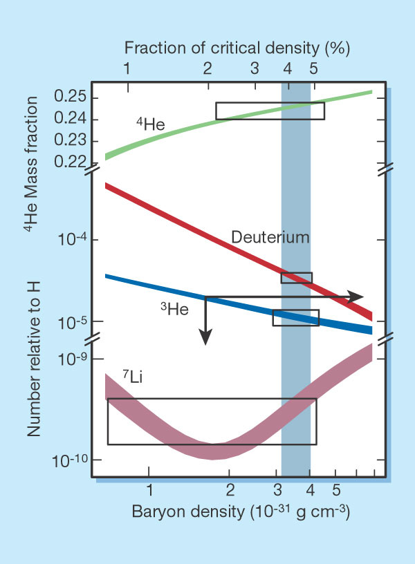
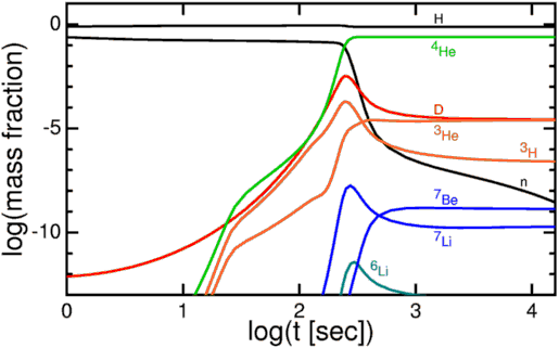
Problems

I Revisiting problem I of chapter 8, now that we know the equilibrium abundance of baryons as in eq. (9.1) and assuming neutral universe $n_e\sim n_p=1.5\times {10}^{-10}{T}^3$, and given that the mass difference or binding energy of Hydrogen is $13.6$eV, what was the ratio at $T=14eV$, and $1.4$eV at $0.14$eV? Determine the temperature when $n_H/n_p=1$ and the universe turned neutral.
II Use Friedman equation to reproduce the temperature-time relation of eq. (9.20) recalling that only photons and neutrinos are relativistic at these temperatures (but with different temperatures!)
III Rewrite the RHS differential equation as $\mathrm{\Gamma }(x)(1+e^{-x})(X_n^{eq}(x)-X_n(x))/H(x)$. Given the initial condition $X(x_i)=X_n^{eq}(x_i)$ show that the solution reads

$X_n(x)$ $=X_n^{eq}(x_i)e^{-(I(x)-I(x_i))}+e^{-I(x)}{\displaystyle {\int }_{x_i}^x}𝑑x^{\prime }{X}^{eq}(x^{\prime }){\displaystyle \frac{dI(x^{\prime })}{d{x}^{\prime }}}{e}^{I(x^{\prime })}$ (9.25)

$I(x)-I(x_i)$ $\equiv {\displaystyle {\int }_{x_i}^x}{\displaystyle \frac{dx}{x}}{\displaystyle \frac{\mathrm{\Gamma }(x)}{H(x)}}(1+e^{-x})$ (9.26)

where in the second term we have cancelled out the dependence on $I(x_i)$. Use integration by parts on the second term to rewrite it as

$X_n(x)$ $=X_n^{eq}(x)-e^{-I(x)}{\displaystyle {\int }_{x_i}^x}𝑑x^{\prime }{\displaystyle \frac{d{X}^{eq}}{d{x}^{\prime }}}{e}^{I(x^{\prime })}$ (9.27)

At late times $x\gg 1$ the equilibrium contribution can be neglected and $I(x)\to 0$ so compute numerically the integral to obtain $X(x\gg 1)=0.15$ (you can take $x_i=0.1$, $\beta =0.385,\mathrm{\Delta }{m}_n=1.293$MeV, $G_F=1.166\times {10}^{-5}$GeV${}^{-2}$ and $g_{\star }=10.75$)

10 Thermal dark matter production

This section turns to dark matter and a possible mechanism for its production in the abundance observed today. Nucleosynthesis provided a valuable check of our theory of the hot early universe since observations could be compared with definite predictions based on our knowledge of all particles and interactions involved; in contrast dark matter remains an unknown substance not composed of any of the particles we know of and whose couplings to matter and to itself are unknown. Applying the thermal production mechanism we just saw at play in BBN to dark matter is therefore an unchecked hypothesis albeit one based on a process which has occurred in nature before. In addition, as is often the case in research, extension of a tested idea to new domains helps us develop a scenario where computations can be made and where enough experimental inputs can prove or disprove the original idea.

The basis for the production of thermal dark matter is the interaction with the primordial plasma as described by Boltzmann equation. As our study of this equation shows the relevant parameters to discuss the outcome are the mass or energy threshold, in this case dark matter mass, and interactions, that is the cross section. We will denote dark matter properties like mass or coupling with a dm subindex.

One important consideration about particle dark matter is that it must be very long lived or completely stable since otherwise it would not stick around long enough to be present today. There are a few examples in nature for inspiration of stable massive particles: the proton is the lightest particle with what we call baryon number and hence stable; the electron is the lightest electromagnetically charged particle so it too is stable. We say they are stable due to symmetry, or explicitly because they are the lightest particle to carry certain conserved number. This too can be applied to dark matter by assuming it has some new conserved quantum number which prevents its decay; for example in supersymmetric extensions of the standard model dark matter is the lightest particle to possess $R$-parity. Here we will assume it is stable or at least ${\tau }_{\mathrm{dm}}>H_0^{-1}$.

10.1 Freeze out

The case that follows closest nucleosynthesis is referred to as dark matter freeze out. One starts with an equilibrium abundance of dark matter $n_{\mathrm{dm}}\sim T^3$ and as temperature drops below the mass of the dark matter particle abundance falls and then freezes at some value once equilibrium is lost.

The reaction responsible for dark matter equilibrium with the primordial bath should respect the symmetries we have imposed on the theory; if we have given dark matter a conserved quantum number as assumed here, it cannot be produced one at a time but instead in an amount with no net quantum number. The simplest case is then that it is produced in particle anti-particle pairs so that assuming $n_{\mathrm{dm}}=n_{\mathrm{anti}-\mathrm{dm}}$

$\mathrm{dm}+(\mathrm{anti}-\mathrm{dm})$ $\leftrightarrow a+b$ (10.1)

${\displaystyle \frac{1}{a^3}}{\displaystyle \frac{d{a}^3{n}_{\mathrm{dm}}}{dt}}=$ ${\left(n_{\mathrm{dm}}^{(0)}\right)}^2⟨\sigma v⟩\left({\displaystyle \frac{n_a{n}_b}{n_a^{(0)}{n}_b^{(0)}}}-{\displaystyle \frac{n_{\mathrm{dm}}^2}{{(n_{\mathrm{dm}}^{(0)})}^2}}\right)$ (10.2)

with particles $a$ and $b$ being either known or other proposed particles but in any case in equilibrium with the bath. This means that the dependence on their abundance and equilibrium abundance cancels out to give

$a^{-3}{\displaystyle \frac{d{a}^3{n}_{\mathrm{dm}}}{dt}}=⟨\sigma v⟩\left({(n_{\mathrm{dm}}^{(0)})}^2-n_{\mathrm{dm}}^2\right)$ (10.3)

which is a closed system for the evolution of dark matter abundance. This simplifies remarkably the production and gives the mechanism part of its appeal in the prediction of abundance as a function of only its couplings $⟨\sigma v⟩$ and mass $m_{\mathrm{dm}}$ given that the initial conditions are set by assuming equilibrium.

It remains then to ready up the equation for solution with the same steps we are already familiar with now defining

$Y\equiv$ ${\displaystyle \frac{n_{\mathrm{dm}}}{T^3}}$ $x=$ ${\displaystyle \frac{m_{\mathrm{dm}}}{T}}$ (10.4)

where $Y$ is the yield which gives roughly the number of dark matter particles per particles in the bath. With these definitions

$xH(x){\displaystyle \frac{dY}{dx}}$ $={\displaystyle \frac{m_{\mathrm{dm}}^3⟨\sigma v⟩}{x^3}}\left(Y_{(0)}^2-Y^2\right)$ (10.5)

$x{\displaystyle \frac{dY}{dx}}=$ ${\displaystyle \frac{\mathrm{\Gamma }(x)}{H(x)}}\left(Y_{(0)}^2-Y^2\right)$ (10.6)

where we defined the rate and equilibrium yield as

$\mathrm{\Gamma }(x)$ $={\displaystyle \frac{m^3}{x^3}}⟨\sigma v⟩$ $Y_{(0)}$ $=g_{\chi }{\displaystyle \frac{x^3}{m^3}}{\displaystyle \int e^{-E/T}\frac{d^{3}p}{{(2\pi )}^3}}={\displaystyle \frac{g_{\chi }}{4{\pi }^2}}{\displaystyle \int z^2𝑑z{e}^{-\sqrt{x^2+z^2}}}$ (10.7)

so that $Y_{(0)}$ is approximately a constant at low $x$ but it decays exponentially at large $x$ signalling that the production of $\chi +{\chi }^{†}$ pairs is no longer energetically viable. In general $\sigma v$ itself depends on $x$ but for renormalizable interactions this dependence is mild for the range of interest and the estimates we derive here will be for constant cross section.

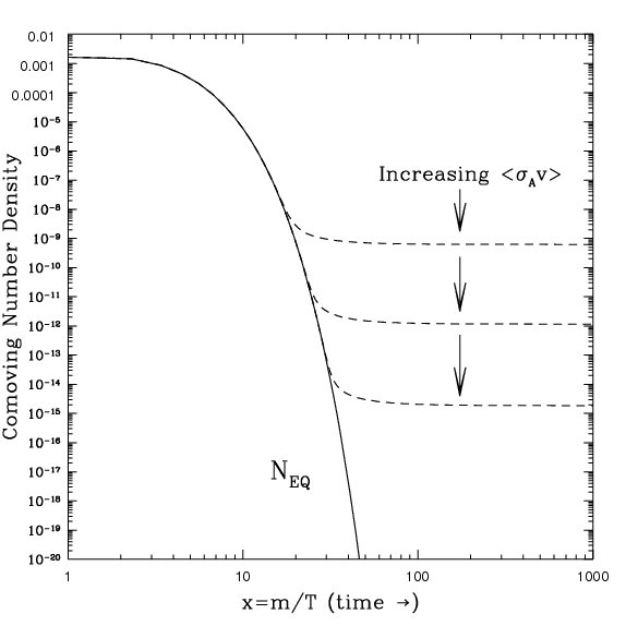
The two limiting behaviours of the abundance are again simple to study. At early times $x\ll 1$ the equilibrium distribution over temperature cube is a constant which makes the RHS in eq. (10.6) vanish in accordance with zero derivative on the LHS, $Y(x)=Y_{(0)}(x)$. As a side comment, although a plot of $Y_{(0)}(x)$ for does not seem constant the derivative on eq. (10.6) is a logarithmic derivative $x\frac{d}{dx}=d/d\log (x)$; in terms of $\log (x)$ the distribution does resemble a constant for , .

At late times or low temperatures $x\gg 1$, the equilibrium yield falls off exponentially and can be neglected to yield an equation

$x{\displaystyle \frac{dY}{dx}}$ $=-{\displaystyle \frac{\mathrm{\Gamma }(x)}{H(x)}}{Y}^2=-{\displaystyle \frac{\lambda }{x}}{Y}^2$ $\lambda$ $={\displaystyle \frac{m⟨\sigma v⟩}{\sqrt{4{\pi }^3{G}_N{g}_{\star }/45}}}$ (10.8)

where given our approximations $\lambda$ is a dimensionless constant which gives the rate to Hubble ratio at $x=1$. This should influence the final abundance in that the largest $\lambda$ the smaller abundance of dark matter particles left. This is simple to see play out in solving the equation to find

${\displaystyle \frac{1}{Y_f}}-{\displaystyle \frac{1}{Y}}$ $={\displaystyle \frac{\lambda }{x}}-{\displaystyle \frac{\lambda }{x_f}}$ $Y(x\gg x_f)\simeq$ ${\displaystyle \frac{x_f}{\lambda }}$ (10.9)

where in the second line we assumed the final abundance is much smaller than that when the distribution deviates from equilibrium $Y_f^{-1}\ll Y^{-1}(x\gg x_f)$ ($Y_f\gg Y(x\gg x_f)$).

This shows the simple inverse relation that gives a larger abundance for weakly coupled particles yet the exact value depends on $x_f$. The differential equation which we are working with now does not have a known analytic solution and so the estimates for $x_f$ rely on numerical studies. An approximation often used which works surprisingly well for its simple-mindedness is to take $x_f=10$ independent of $\lambda$, in the problem set you can derive a more precise relation yourself. Then we have a yield frozen out in the value

$Y(x\gg x_f)$ $={\displaystyle \frac{x_f}{\lambda }}$ $n_{\mathrm{dm}}$ $={\displaystyle \frac{x_f}{\lambda }}T{(x)}^3={\displaystyle \frac{x_f}{\lambda }}T{(x_1)}^3{\displaystyle \frac{a{(t_1)}^3}{a{(t)}^3}}$ (10.10)

where we express it in terms of the scale factor rather than temperature since as we have seen already the scaling $T\propto a^{-1}$ is not followed when going through thresholds.

This is relevant since the abundance of dark matter is measured today as

${\rho }_{\mathrm{dm}}=m_{\mathrm{dm}}{n}_{\mathrm{dm}}(t_0)=0.27{\rho }_{\mathrm{cr}}=1.3{\left({\displaystyle \frac{h}{0.67}}\right)}^2{\displaystyle \frac{\mathrm{KeV}}{{\mathrm{cm}}^3}}$ (10.11)

so we evolve the abundance with a bit of trickery as

${\rho }_{\mathrm{dm}}(t)={\displaystyle \frac{m_{\mathrm{dm}}{x}_f}{\lambda }}{T}_1^3{\displaystyle \frac{a{(t_1)}^3}{a{(t)}^3}}=m_{\mathrm{dm}}{\displaystyle \frac{x_f}{\lambda }}{T}_0^3{\left({\displaystyle \frac{a_1{T}_1}{a(t)T(t)}}\right)}^3=m_{\mathrm{dm}}{\displaystyle \frac{x_f}{\lambda }}{T}_0^3{\displaystyle \frac{g_{\star }(t)}{g_{\star }(t_1)}}$ (10.12)

where there is a dependence on the relativistic degrees of freedom by decoupling time. One can write the equation above in terms of the cross section and with appropriate units as

${\left({\displaystyle \frac{h}{0.67}}\right)}^2{\mathrm{\Omega }}_{\mathrm{dm}}={\displaystyle \frac{2x_f}{\sqrt{g_{\star }}}}{\displaystyle \frac{{10}^{-38}{\mathrm{cm}}^2}{⟨\sigma v⟩}}$ (10.13)

where the mass drops out (neglecting the mild dependence in $g_{\star }$). So the right abundance would be reproduced for a cross section around femtobarn (barn=${10}^{-24}$cm${}^2$), this value is familiar from collider physics with this being the typical weak process cross section, to be precise this weak cross section would involve the mass too as $G_F^2{m}_{\chi }^2$ so the mass of dark matter if the interaction is the weak force would be 10 GeVish. The fact that the choice of values which are around typical weak cross section (like that of the neutrino and proton to neutron conversion) and electroweak scale masses was taken to be a strong indication for models of WIMP dark matter, like those based on supersymmetry, going as far as to call it a miracle. It is indeed strong theoretical evidence, (although divine intervention not needed), that the solution to two independent open problems in physics, i.e. electroweak hierarchy problem and dark matter points towards particles of the same mass/couplings.

10.2 Freeze-in

We can revisit our initial conditions to find a thermal production mechanism with qualitative different features while still described by Boltzmann equation. The freeze out mechanism described above assumed an initial equilibrium abundance; this is a plausible possibility since as we have seen the equilibrium solution is locally an attractor and we believe that all standard model particles used to be in this state. For the standard model particles this was derived considering their typical couplings, $\sim \alpha$, as compared to the Hubble rate so for temperatures $T_{\mathrm{eq}}\sim 4\pi {\alpha }^2{M}_{\mathrm{Pl}}\sim {10}^{16}$GeV and below an equilibrium abundance $\sim T^3$ was reached. However for dark matter we do not know what is the value of the couplings but what we can say is that the smaller it is, the longer it would take to attain equilibrium $T_{\mathrm{eq}}\sim 4\pi {\alpha }_{\mathrm{dm}}^2{M}_{\mathrm{Pl}}$. In particular if this temperature is smaller than the mass of the dark matter particle equilibrium is never attained since by temperature $T_{eq}$ the production is not energetically viable. So roughly speaking

${\alpha }_{\mathrm{dm}}^2{M}_{\mathrm{Pl}}$ $>m_{\mathrm{dm}}$ equilibrium is attained (10.14)

${\alpha }_{\mathrm{dm}}^2{M}_{\mathrm{Pl}}$ equilibrium is not attained (10.15)

Figure 14: Freeze in

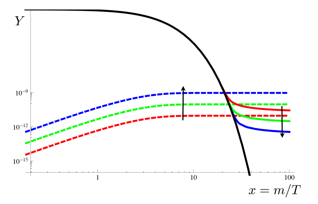
The second possibility follows from feeble (i.e. small) couplings and is what we explore next. Although there are a few possibilities for the reaction that produces feeble dark matter including three body interactions, here we will take the one closest to what we have done thus far in the reaction $C+\chi \to A+B$ where all particles $A,B,C$ are in thermal equilibrium with the bath. For simplicity we take dark matter to be the only relevant mass of the four particles.

The basic tools to describe this scenario we have now used a good number of times, Boltzmann equation reads

$a^{-3}{\displaystyle \frac{d{a}^3(t)n_{\mathrm{dm}}}{dt}}=n_{\mathrm{dm}}^{(0)}{n}_C^{(0)}⟨\sigma v⟩\left(1-{\displaystyle \frac{n_{\mathrm{dm}}}{n_{\mathrm{dm}}^{(0)}}}\right)$ (10.16)

Our customary refurbishment of the equation gives

$x{\displaystyle \frac{dY}{dx}}={\displaystyle \frac{n_C(x)⟨\sigma v⟩(x)}{H(x)}}\left(Y_{(0)}-Y\right)\equiv {\displaystyle \frac{\mathrm{\Gamma }(x)}{H(x)}}\left(Y_{(0)}-Y\right)$ (10.17)

This is a linear inhomogeneous first order equation and hence we can solve it exactly, nonetheless given our assumption of equilibrium never quite reached one does not even need the full solution. Neglecting $Y$ in the RHS which is assumed never reaches $Y_0$ before $x=1$ one can approximate

$x{\displaystyle \frac{dY}{dx}}$ $={\displaystyle \frac{\mathrm{\Gamma }}{H}}{Y}_{(0)}$ $Y(x)$ $={\displaystyle \int \frac{dx}{x}\frac{\mathrm{\Gamma }}{H}{Y}_{(0)}}$ (10.18)

Given that $Y_{(0)}\sim g_{\star \chi }{\pi }^2/30$ for $x\ll 1$ and $Y_{(0)}\sim e^{-x}$ for $x\gg 1$ we can further approximate it to a step function whereas taking the cross section to be $\sigma v\sim 4\pi {\alpha }_{\mathrm{dm}}^2/T^2$ one obtains

$Y(x)\simeq g_{\chi }{g}_C{\left({\displaystyle \frac{{\pi }^2}{30}}\right)}^2{\displaystyle \frac{M_{\mathrm{Pl}}4\pi {\alpha }_{\mathrm{dm}}^2}{m_{\mathrm{dm}}\sqrt{4{\pi }^3{g}_{\star }/45}}}{\displaystyle \int 𝑑x\mathrm{\Theta }(x_{fi}-x)}$ (10.19)

So in this rough picture the abundance initially grows linearly with $x$ up until $x=x_{fi}$ when it reaches a plateau. The actual shape can be appreciated in fig. 14.

Converting the yield to present day energy density involves the same manipulation of scale factors and temperature as for freeze out so one has:

${\rho }_{\mathrm{dm}}(t)=m_{\mathrm{dm}}Y(x\gg x_{fi})T_0^3{\displaystyle \frac{g_{\star }(t)}{g_{\star }(t_1)}}=g_{\mathrm{dm}}{g}_C{\left({\displaystyle \frac{{\pi }^2}{30}}\right)}^2{\displaystyle \frac{M_{\mathrm{Pl}}4\pi {\alpha }_{\mathrm{dm}}^2{x}_{fi}}{m_{\mathrm{dm}}\sqrt{4{\pi }^3{g}_{\star }/45}}}{T}_0^3{\displaystyle \frac{g_{\star }(t)}{g_{\star }(t_1)}}$ (10.20)

which gives an relative contribution of

${\mathrm{\Omega }}_{\mathrm{dm}}=2.6\left({\displaystyle \frac{2x_{fi}{g}_{\mathrm{dm}}{g}_C}{g_{\star }^{3/2}}}\right)\left({\displaystyle \frac{4\pi {\alpha }_{\mathrm{dm}}^2}{{10}^{-28}}}\right)$ (10.21)

which again is independent of the dark matter mass while the prefactor point to the right relic abundance for a very small coupling ${\alpha }_{\mathrm{dm}}\sim {10}^{-15}$.

Finally one can synthesize the two mechanisms in terms of the same variables with $⟨\sigma v⟩(x_{fi})=4\pi {\alpha }_{\mathrm{dm}}^2/m_{\mathrm{dm}}^2$ so that

$Y\sim$ ${{\displaystyle \frac{H}{\mathrm{\Gamma }}}|}_{x_f}\sim {\displaystyle \frac{1}{m_{\mathrm{dm}}{M}_{\mathrm{Pl}}⟨\sigma v⟩(x_f)}}$ Freeze out (10.22)

$Y\sim$ ${{\displaystyle \frac{\mathrm{\Gamma }}{H}}|}_{x_{fi}}\sim m_{\mathrm{dm}}{M}_{\mathrm{Pl}}⟨\sigma v⟩(x_{fi})$ Freeze in (10.23)

which can be regarded as the outcome when expanding on a small parameter, a small rate of interactions over Hubble for freeze in or a small Hubble over the interaction rate for freeze out. Note that in both cases yield is proportional to the small parameter and $Y\ll 1$. At the same time, a valuable property that these mechanisms share is the independence on the initial time/ temperature $x_i$ where one assumes the evolution starts.

Problems

I Substitute in eq. (10.13) $\sigma v=G_F^2{m}_{\mathrm{dm}}^2$ and find the mass of dark matter as a function of $x_f$, $g_{\star }$
II For eq. (10.21) of the freeze in substitute $4\pi {\alpha }_{\mathrm{dm}}^2=m_{\mathrm{dm}}^2⟨\sigma v⟩$ and derive a cross section mass relation, for a cross section around ${10}^{-12}$ab with ab$={10}^{-15}$b and b$={10}^{-24}$cm${}^2$ what would dm mass be? You can take $g_{\star }=106.75$
III A more accurate estimate of the freeze out time is $x_f$ such that

$n^{(0)}(x_f)⟨\sigma v⟩=H(x_f)$ (10.24)

substitute in the equilibrium abundance for a non relativistic particle to find the explicit equation for $x_f$.
IV Both freeze in and out predict small yield $Y$, can you recall any instance in which a particle retains an order one yield after decoupling? If we use this third case to produce dark matter what would be the approximate mass required (you can neglect changes in $g_{\star }$)?

11 Inflation

Experimental evidence shows that Einstein field equations describe the dynamics of the universe back to a hot bath of particles of temperature at least $T\sim$MeV when the expansion was dominated by radiation. One can take the scale factor for this period, that is for as:

$a(t)={\displaystyle \frac{1}{z_{eq}}}{\left({\displaystyle \frac{t}{2.1\times {10}^{12}\mathrm{s}}}\right)}^{1/2}$ (11.1)

so matter-radiation equality occured when the universe was about hundred thousand years old. Radiation domination at early enough times is a consequence of the scaling with $a$ of its energy density ${\rho }_r$ being the most steep of the known substances; it would seem reasonable then to extrapolate radiation domination back to arbitrarily small time $t\to 0$. If we do this however we run into the horizon problem.

Recall from sec. 3 that events that ocurred in opposite directions in the sky at time $t$ and whose light is reaching us now could have been in causal contact or not depending on

$\eta (t)\ge$ $\mathrm{\hspace{0.17em}}\eta (t_0)/2\mathit{\hspace{1em}}\text{causally connected}$ (11.2)

$\mathrm{\hspace{0.17em}}\eta (t_0)/2\mathit{\hspace{1em}}\text{causally disconnected}$ (11.3)

Take for example two photons from the CMB, decoupling occured at $t_{*}\sim$380.000y a bit into the matter era, taking this into account and computing $\eta (t_{*})$ as (explicitly we take $z_{*}\sim {10}^3$)

${\displaystyle {\int }_0^{t_{*}}}$ ${\displaystyle \frac{dt}{a(t)}}=0.075H_0^{-1}\simeq {10}^{9}y$ ${\displaystyle {\int }_0^{t_0}}$ ${\displaystyle \frac{dt}{a(t)}}\sim 3.2H_0^{-1}\simeq 60\times {10}^{9}y$ (11.4)

The ratio is much less than 1/2 so these two photons had not been in causal contact, how come then the temperature of the CMB is the same in all directions to one part in a hundred thousand?

11.1 Solving the horizon problem

To restore causality we have to give up our extrapolation of radiation domination all the way back to $t=0$ and substitute it by another $a(t)$ behaviour. In order to make the events we see in the sky causally connected we should push them into the upper half of $\eta (t_0)$, which can be accomplished if we make $\eta$ grow much faster than ordinary time in an early phase. In other words, make the first integral in eq. (11.4) for some early time interval much larger than the interval itself, inflate it. As to how much larger, given that the universe is radiation dominated at least as early as BBN ($t\sim 1$s), we want the conformal time for an event at some time $t_e$ smaller than a second to be already larger than half $\eta (t_0)=3.2H_0^{-1}=3.4t_0$, i.e.

${\displaystyle {\int }_0^{t_e}}{\displaystyle \frac{dt}{a(t)}}\ge {\displaystyle \frac{3.4}{2}}{t}_0$ (11.5)

Let us cast this in a slightly more readable from as

${\displaystyle \int \frac{da}{a}\frac{a_e{H}_e}{aH}}\ge a_e{H}_e{\displaystyle \frac{3.4}{2}}{t}_0\simeq {10}^8\sqrt{{\displaystyle \frac{\mathrm{s}}{t_e}}}$ (11.6)

where for $a_{e}H(t_e)$ we used the radiation domination formula assuming the universe has just started that phase. The integral on the LHS has a first term which is $d\log a$ and so the contribution during an e-fold $a(t)/a(t^{\prime })=e$ in the integral is roughly given by the remaining integrand if it can be taken as a constant. The integral must yield a hierarchy of at least 8 orders of magnitude, in reality, typical models solving the horizon problem operate so early ($t\sim {10}^{-32}-{10}^{-40}$s) that the number of orders of magnitude to be accounted for are 50 or 60 e-folds; what could possibly produce such a hierarchy?

A very mild requirement for this integral to be much larger in the past is to have the integrand be larger the further back in time or smaller a, that is

${\displaystyle \frac{d}{dt}}$ ${\displaystyle \frac{d}{dt}}{\displaystyle \frac{1}{\dot{a}(t)}}$ (11.7)

That implies accelerated expansion $d^{2}a/d{t}^2>0$; none of radiation, matter or even curvature can reproduce this behaviour but we have encountered a case that does the job.

Assume then an epoch of cosmological constant domination, we would then have

$a(t)=a(t_e)$ $e^{\sqrt{{\mathrm{\Lambda }}_I/3}(t-t_e)}$ $t$ (11.8)

Then the conformal time integral reads

$a_e{H}_e{\displaystyle \int \frac{dt}{a(t)}}=H_e{\displaystyle {\int }_{t_i}^{t_e}}𝑑t{e}^{H_I(t_e-t)}={\displaystyle \frac{H_e}{H_I}}\left(e^{H_i(t_e-t_i)}-1\right)$ (11.9)

If one approximates the Hubble rate at the end and during the acceleration to be approximately the same the expression simplifies to

$\simeq e^{H_I\mathrm{\Delta }t}={\displaystyle \frac{a(t_e)}{a(t_i)}}>{10}^{22}\sqrt{{\displaystyle \frac{{10}^{-32}\mathrm{s}}{t_e}}}\sim {10}^{10}{\displaystyle \frac{T}{\mathrm{MeV}}}$ (11.10)

Hence one can account for the large hierarchy with an exponential of the fundamental parameters of the theory, it suffices that the time interval last some 60 times the Hubble time during inflation. In terms of universe growth it has to be in an accelerated phase for that many efolds, i.e it inflated by a factor of ${10}^{27}$. Note that we were lead to this solution by the mild condition of eq. (11.7).

Figure 15: Inflating a to solve the horizon problem, the blue and red areas are supposed to be the same

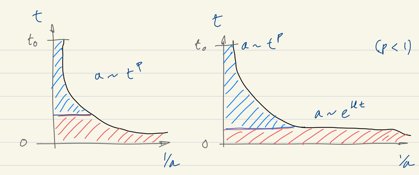
We turn next to the implementation of this mechanism in quantum field theory.

11.2 Realization from QFT

One of the differences with the accelerated expansion we have today and the phase which might have happened at very early times is that the latter has to end and give way to radiation domination. Another quantitative difference is that the cosmological constant during inflation and nowadays differs by many, many orders of magnitude (see problem sheet). These differences point towards something not as ‘simple’ as a cosmological constant, so one should explore the possibility of a transient very large cosmological constant.

To explore this possibility we look into the evolution of the universe when Hubble is dominated by a the energy density from a scalar field with a potential. We only know of one (possibly) elemental scalar field in nature which could play this role, the Higgs boson. Nevertheless the Standard Model as we know it does not have the right couplings to produce inflation so here we will assume our scalar is another scalar particle, conventionally called the inflaton $\varphi$. We derive our dynamics from the action:

${\displaystyle \int d^{4}x\sqrt{|g|}\left(-\frac{R}{16\pi G_N}+\frac{1}{2}{\partial }_{\mu }\varphi {\partial }^{\mu }\varphi -V(\varphi )\right)}$ (11.11)

This action has a energy-momentum tensor:

$T_{\mu \nu }={\partial }_{\mu }\varphi {\partial }_{\nu }\varphi -g_{\mu \nu }[{(\partial \varphi )}^2/2-V(\varphi )]$ (11.12)

so that Einstein field equations together with the scalar EOM

$R_{\mu \nu }-{\displaystyle \frac{1}{2}}{g}_{\mu \nu }R$ $=8\pi G_N\left(-{\displaystyle \frac{2}{\sqrt{|g|}}}{\displaystyle \frac{\delta }{\delta g_{\mu \nu }}}\sqrt{|g|}{ℒ}_{\varphi }\right)$

$=8\pi G\left({\partial }_{\mu }\varphi {\partial }_{\nu }\varphi -g_{\mu \nu }[{(\partial \varphi )}^2/2-V(\varphi )]\right)$ (11.13)

${\nabla }_{\mu }{\partial }^{\mu }\varphi$ $=-V^{\prime }(\varphi )$ (11.14)

Substituting in now our beloved homogeneous approximation for the metric and scalar field as $\varphi =\varphi (t)$, ${\partial }_{\mu }\varphi =(\dot{\varphi },0)$.

(11.15)

Where the associated energy density and pressure can be read off. In particular one sees that if the potential term dominates (and is positive) there could be negative pressure and a phase of acceleration.

The EOM with the homogeneous ansatz collapse to three equations

$3H^2$ $=8\pi G({({\partial }_t\varphi )}^2/2+V(\varphi ))$ (11.16)

$-3H^2-2\dot{H}$ $=8\pi G({({\partial }_t\varphi )}^2/2-V(\varphi ))$ (11.17)

$\ddot{\varphi }+3H\dot{\varphi }=$ $-V^{\prime }(\varphi )$ (11.18)

were Einstein field equations can be linearly combined into

$H^2=$ ${\displaystyle \frac{8\pi }{3}}{G}_N\left({\displaystyle \frac{{\dot{\varphi }}^2}{2}}+V(\varphi )\right)$ $\dot{H}$ $=-4\pi G_N{(\dot{\varphi })}^2$ (11.19)

If an accelerated expansion takes place the $H^2$ term dominates and is approximately constant which is to say a small ratio $ϵ$

$ϵ\equiv {\displaystyle \frac{-\dot{H}}{H^2}}$ (11.20)

so one of the conditions for inflation is $ϵ\ll 1$. Nonetheless one shall inspect the EOM for $\varphi$ also to ensure that a constant value of $\varphi$ to yield a constant $V(\varphi )$ is dynamically viable. The EOM for $\varphi$ resembles a point mass in one dimension subject to a potential but in a viscous substance that adds drag $H$. The field can then move slowly if the drag dominates over the kinetic term. This gives the second condition for inflation, which is for it to last enough, the $\varphi$ EOM should be dominated by the friction term, i.e.

$\delta \equiv -{\displaystyle \frac{\ddot{\varphi }}{H\dot{\varphi }}}$ (11.21)

should also be small. If it is indeed small and so is $ϵ$ one can approximate:

$3H\dot{\varphi }$ $\simeq -V^{\prime }$ $ϵ$ $\simeq {\displaystyle \frac{3{\dot{\varphi }}^2}{2V}}={\displaystyle \frac{V^{\prime 2}}{6H^{2}V}}={\displaystyle \frac{1}{16\pi G_N}}{\left({\displaystyle \frac{V^{\prime }}{V}}\right)}^2$ (11.22)

$3\dot{H}\dot{\varphi }+3H\ddot{\varphi }$ $\simeq -V^{\prime \prime }\dot{\varphi }$ $-3$ $ϵ-3\delta \simeq -{\displaystyle \frac{V^{\prime \prime }}{H^2}}=-{\displaystyle \frac{3}{8\pi G_N}}{\displaystyle \frac{V^{\prime \prime }}{V}}$ (11.23)

While the two conditions $\delta ,ϵ\ll 1$ are satisfied there will be an inflationary phase.

Nonetheless, inflation has to end too! One can estimate the duration of inflation from the potential, and it should be such that the growth of the scale factor is the huge value given earlier, so let us write

$N_{\text{e-folds}}=51-{\displaystyle \frac{1}{2}}\log \left({\displaystyle \frac{t_e}{{10}^{-32}\mathrm{s}}}\right)={\displaystyle \int H(t)𝑑t}={\displaystyle \int \frac{H}{\dot{\varphi }}𝑑\varphi }={\displaystyle {\int }_{{\varphi }_i}^{{\varphi }_e}}{\displaystyle \frac{\sqrt{4\pi G_N}}{\sqrt{ϵ}}}𝑑\varphi$ (11.24)

where ${\varphi }_i$ is the value of the field at the beginning of inflation and the fvalue at the end we determine from ${\varphi }_e=\varphi (t_e)$

${\displaystyle \frac{M_{\mathrm{Pl}}{V}^{\prime }({\varphi }_e)}{V({\varphi }_e)}}\simeq 1$ (11.25)

The scenario we described is referred to as slow roll yet this might be quite misleading if using our intuition for balls rolling down slopes; the physical system here does not have quite the same dynamics, for one the Hubble friction depends on the potential itself and is larger the higher $V$ so for example a ${\varphi }^2$ potential which you might think is too step can do the job.

These are the basic dynamics of inflation at the homogenous and isotropic level, we have seen that there is the possibility of a scalar field stuck in a constant value for some period and eventually accelerating out of this phase. The inflationary phase is so violent that dilutes all possible initial abundances and possible curvature; the latter is actually a convenient by-product since as we know the universe is observed to have no curvature. As for the dilution of all particle abundances, this poses a potential problem since the universe should enter a hot radiation era after inflation; the abundance of standard model particles should increase up to their equilibrium abundances. This is assumed to happen in the re-heating period when the inflaton decays and produces Standard Model particles. Although successful reheating is not guaranteed and deserves its own study here we shall not go any deeper into it.

11.3 Initial perturbations

Figure 16: Bounds on inflation parameters primoridal tilt $n_s=1-6ϵ+4\delta$ and tensor-to-scalar ratio $r=16ϵ$ for different models.

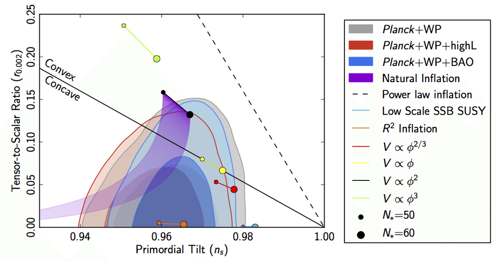
The uses of inflation extend beyond solving the horizon problem which lends further credibility to the theory. Inflation also provides the initial perturbations that seeded the distribution of matter as we observe it today. One of the consequences of the violence of inflation is that the causality of general relativity interferes with quantum mechanics.

Vacuum fluctuations of momentum $\mathrm{\Delta }p$ are allowed by the uncertainty principle to live within a distance $\mathrm{\Delta }x\sim \mathrm{\hslash }\mathrm{\Delta }p$, however inflation is stretching out space and does it so fast that it might causally disconnect the region $\mathrm{\Delta }x$. In that case the perturbation cannot evolve in time any longer and is said to be frozen out or grown larger than the horizon. The basis for this prediction is then the computation of the spectrum for vacuum oscillations, but this has to be computed in a de-Sitter vacuum $|$dS$⟩$, that is, an accelerating universe

$⟨\mathrm{dS}|\varphi (x)\varphi (y)|\mathrm{dS}⟩$ (11.26)

You might be familiar with this object in the case of QFT with a Minkowski vacuum; it is the field propagator or two point function $\sim \int d^{4}k{e}^{ik(x-y)}/(p^2-m^2)$. The computation here requires quantization in curved space time; the tools to carry it out we have not acquired yet so we will not reproduce the result here. The promise of this computation is awe inspiring in its ambition nevertheless: to account for the seeds of the universe as we know it, us included. The production of these initial perturbations can be compared with the inhomogeneities and anisotropies observed today and although the theory has indeed passed some non-trivial tests at the moment we do not know much about the potential of inflation and we have not stress tested the theory. Measurements of homogeneities can be translated to parameters of inflation, namely combinations of $ϵ$ and $\delta$ as reported in fig 16.

Problems

I Present conformal time, assuming no inflationary phase is given by late times and is approximately $\eta (t_0)=3.2H_0^{-1}$. Compute $\eta (t_{1/2})=\eta (t_0)/2$ assuming you can take a matter dominated universe for the whole integration interval. What is the redshift and CMB temperature for $t_{1/2}$? Had decoupling occured ($T_{*}\sim 0.3$eV)?
II Take the potential to be a mass term $V(\varphi )=m^2{\varphi }^2/2$ and compute $ϵ,\delta$. For small paremeters does the value of the field have to be above or below $M_{\mathrm{Pl}}$? For that value is $H$ above $M_{\mathrm{Pl}}$? Compute the e-folds in eq. (11.24) taking ${\varphi }_e$ from eq. (11.25), and write it as a function of $ϵ({\varphi }_i)$. If we approximate $ϵ$, $\delta$, during inflation to be evaluated at this slow rolling value ${\varphi }_i$ we have a predition for $n_s$ and $r$, where do they fall in fig16 (take $N\sim$ 50 and 60).

12 Cosmology as a field theory

The smooth hot expanding universe study has produced a number of tested predictions that confirmed the theory together with other untested yet plausible ones as we have seen in the previous lectures. We have indeed managed to learn a good deal and to turn back the dial of time to find what the universe used to look like to a good approximation.

This description nonetheless does not account for the fact that the universe is not exactly the same everywhere and the stress energy tensor and curvature vary from place to place, even at the largest scales.

Nonetheless both at the largest scales and at early times this space dependence of energy density and curvature is a small correction, in the order of one part in a hundred thousand, which means we can roll out the familiar machinery of perturbation theory. Even in the regime in which perturbation does not hold, like in structure formation, one can resort to numerical solutions and simulations, although we won’t cover these here.

Moving into this more detailed examination of the cosmos it is important to highlight a distinction. There will be aspects of what we see that we cannot account for like why does our group of galaxies contain a few dozen; what theory will be able do is trace back our current situation in time or give us how big are groups of galaxies on average.

This is to say, as we resolve spatial distributions, one makes use of statistical physics to treat the data whereas on the theory side full fledged quantum field theory in curved space time is put to use.

12.1 Perturbation theory for Cosmology

The advantage of perturbation theory is that the groundwork has been laid down with our first order study of the universe and we’ve made the journey once from theory to experiment. Now one needs only trace back our steps and add in a small space-dependent modification. In practice the algebra will get considerably more complicated, partly because we are aiming at describing more complex experimental data, partly due to the need to revisit our variables with new terms in our metric and the structure of general relativity.

So one starts from a metric with small deviations $\mathrm{\Psi },\mathrm{\Phi },B,h$ from FRW as:

(12.1)

where $\overline{g}$ is the metric we have been working with thus far $\overline{g}=$Diag$(1,-a,-a,-a)$. Filtering this through the machinery of Riemannian geometry and keeping only linear terms in the perturbations

${\mathrm{\Gamma }}_{\nu \rho }^{\mu }$ $={\overline{\mathrm{\Gamma }}}_{\nu \rho }^{\mu }-\delta g^{\mu {\mu }^{\prime }}{\overline{\mathrm{\Gamma }}}_{{\mu }^{\prime }\nu \rho }+{\overline{g}}^{\mu {\mu }^{\prime }}{\displaystyle \frac{1}{2}}\left({\partial }_{\{\nu }\delta g_{{\mu }^{\prime }\rho \}}-{\partial }_{{\mu }^{\prime }}\delta g_{\nu \rho }\right)$ (12.2)

$R$ $=\overline{R}+\delta R$ (12.3)

to arrive at modified Einstein field equations

$\delta R_{\mu \nu }-{\displaystyle \frac{\overline{R}}{2}}\delta g_{\mu \nu }-{\displaystyle \frac{\delta R}{2}}{\overline{g}}_{\mu \nu }=8\pi G_N\delta T_{\mu \nu }$ (12.4)

The LHS can be obtained following a familiar yet now computationally intensive procedure.

The decomposition theorem tells us that perturbation with different space indices, that is to to say on different representations of the subgroup of rotations of the Lorentz group, evolve independently at the linear level. For simplicity we focus on the scalar perturbations next yet we note that the two-index (traceless) object $h_{ij}$ describes possible gravitational wave perturbations.

The RHS of Einstein field equations nonetheless must be revised as well and to do so we go back to Boltzmann equations. For a collisionless set of particles the distribution function change with time at some phase-space point $p,x$ is given by the particles that ’move into’ $(x,p)$ minus the particles that leave it. The particles that move in were at position $x-v\delta t$ and momenta $p-dp/dt\delta t$ an instant $\delta t$ before so the change in the distribution function:

$\delta f$ $=f(x-{\displaystyle \frac{dx}{dt}}\delta t,p-{\displaystyle \frac{dp}{dt}}\delta t)-f(x,p)$ (12.5)

${\displaystyle \frac{\partial f}{\partial t}}$ $=-{\displaystyle \frac{dx}{dt}}{\displaystyle \frac{\partial }{\partial x}}f-{\displaystyle \frac{dp}{dt}}{\displaystyle \frac{\partial }{\partial p}}f$ (12.6)

Or in other terms total derivative $df/dt=0$. This follows from any system whose dynamics are given by a Hamiltonian (itself coming from a Lagrangian) and the statement that the distribution function has zero total time derivative follows from Liouville’s theorem.

Nonetheless in our system there are collisions and the expansion of the universe makes the definition of our variables not evident a priori. In particular recall that the momentum satisfies, for a particle of mass m:

$g_{\mu \nu }{P}^{\mu }{P}^{\nu }=(1-\mathrm{\Psi }){(P^0)}^2-a^2(1+2\mathrm{\Phi })P^i{P}^j{\delta }_{ij}=m^2$ (12.7)

it is conventional to define

$p^2$ $=a^2(1+2\mathrm{\Phi }){(P^i)}^2$ $E^2$ $=(1+2\mathrm{\Psi }){(P^0)}^2$ (12.8)

and find that, after some algebra and chain rules

${\displaystyle \frac{\partial f}{\partial t}}-{\displaystyle \frac{v^i}{a}}{\displaystyle \frac{\partial f}{\partial x^i}}-E\left({\displaystyle \frac{v}{a}}\nabla \mathrm{\Psi }+v^2(H^2+{\partial }_t\mathrm{\Phi })\right){\displaystyle \frac{\partial f}{\partial E}}=C[f]$ (12.9)

where obtaining this equation required the modified geodesic equation, we changed to polar coordinates in $p^i$, changed the derivative wrt to the modulus $p$ to the energy $E$ variable and neglected derivatives wrt the angle since they give a second order term. The RHS will depend on what species and regime one is looking at, e.g. for photons after $e^{+}{e}^{-}$ annihilation the relevant interaction is Compton scattering.

One can then close the system with

$6H\left({\partial }_t\mathrm{\Phi }-H\mathrm{\Psi }\right)-2{\displaystyle \frac{{\nabla }^2}{a^2}}\mathrm{\Phi }=8\pi G_N\rho \delta$ (12.10)

where we expanded the energy density as $\rho =\rho (1+\delta )$. Two simplifications help see clearly the physics at play, Fourier transforming on $x$ to $k$ (not to confuse with $p$) one realizes the PDE’s go to independent ODE’s.

$\mathrm{\Phi }(x,p)={\displaystyle \int \frac{d^{3}k}{{(2\pi )}^3}{e}^{ikx}\tilde{\mathrm{\Phi }}(k,p)}$ (12.11)

and second all space derivatives in co-moving coordinates come with $1/a$ we can simplify this t-dependence by using conformal time instead.

All in all the distribution function equation takes the schematic form

${\displaystyle \frac{d}{d\eta }}\tilde{f}+ik\cdot {\displaystyle \frac{p}{E}}\tilde{f}=aC[f]+J$ (12.12)

where $J$ is a source term linear in the remaining perturbations and the collision term $C[f]$ which we did not make explicit is nonetheless expanded to be linear in $\tilde{f}$. A word of warning about the literature is that the tilde to denote Fourier transform is often dropped.

Without being explicit and solving differential equations, the behaviour of the solutions can be understood from two observations:

• First the linearity means all different $k$-modes evolve independently, that is, an initial distribution $f({\eta }_0,k)={\delta }^3(k-k_0)$ will maintain it’s monochromatic shape. This is true to our linear approximation, where we can use our intuition of quantum mechanics, or linear superposition to understand that the modes evolve differently.

• The solution to the homogeneous collision-less part, is

  $f=C{e}^{-ik\mu \eta }$ $\mu$ $=k\cdot v=k\cdot {\displaystyle \frac{p}{E}}$ (12.13)

  where we note that for modes $k$ with $k\eta \ll 1$ there is no time evolution

  $\eta k\ll 1\mathit{\hspace{1em}\hspace{1em}}\eta \ll 2\pi L\mathit{\hspace{1em}\hspace{1em}}{e}^{ik\eta }\sim \text{constant}$ (12.14)

  This does indeed match one’s intuition from causality. The perturbation on scales $L$ larger than the horizon, are static up until causal physics can operate. The fact that this behaviour can be accounted for with causality means that the conclusions are more general and apply to the general solution.

We have seen therefore that conformal time and Fourier analysis significantly clarify the evolution of perturbations and allow for distinction of two regimes as dictated by causality.

12.2 Observational data

One can look experimentally for inhomogeneities and anisotropies in a number of ways. If looking at matter distributions one has

${\delta }_m(x)={\displaystyle \frac{{\rho }_m(x)-⟨{\rho }_m⟩}{⟨{\rho }_m⟩}}$ (12.15)

Matter is nonetheless predominantly dark, an observational difficulty which is overcome by assuming baryonic matter follows dark matter or looking at the gravitational influence of dark matter like lensing effects. Let us assume then that via galaxy surveys or other means we resolve a 3-dimensional spatial distribution of matter in the universe. Then contrast with theory of this distribution is not yet straight forward; as we outlined, theory cannot predict that an overdensity will develop here or there and one should look instead at averaged or relative magnitudes. A way of doing this while maintaining a 3-dimensional data set is to look at correlations of the field squared, these will depend on the relative distance with enough statistics:

$⟨⟨\delta (x)\delta (y)⟩⟩=G(|x-y|)$ (12.16)

Where, at the risk of being pedantic we introduced double angle’s to signify averaging over distributions. It must indeed be so for the RHS to match the LHS, since every single element in the average in the LHS is a the product of a function of $x$ and a function of $y$ but the outcome on the RHS is a function of the difference $x-y$.

This brings us to statistics and the ‘problem’ of having one universe only to look at (this is the way physicist actually think). This problem is only acute at the largest scales nonetheless, if one is interested in say $k\sim 10$ Mpc${}^{-1}$ scales and below in our Gpc sized visible universe one can chop up the distribution into ${(1000/10)}^3$ boxes and take each one as a different distribution so that there is enough statistics to obtain a meaningful correlation. It is then at the largest scales where having one universe only means we do not have enough data to compute eq. (12.16). This statistical limitation is at times referred to as cosmic variance. At the same time going to smaller scales, larger $k$, we deal with perturbations which have undergone more processing to form structure like clusters of galaxies and have enter a non-linear regime. This makes extraction of the original perturbations at earlier times a more complicated problem. It is for this reason that when testing the for largest scales of smaller $k$ is a more direct probe of early-time conditions like inflation.

This wave-number discussion is also good to delimit the validity of perturbation theory and the scales at which it breaks down and structure forms which is very interesting on itself.

Given our preference for Fourier analysis, the conventional definition for field-squared correlations is given instead in wave-number space in terms of the power spectrum $P$ as:

$⟨⟨\tilde{\delta }(k)\tilde{\delta }(k)⟩⟩=P(|k|){(2\pi )}^3{\delta }^3\left(k-k^{\prime }\right)$ (12.17)

Much of the talk in cosmology is about this function $P$, the power spectrum and to what degree is it scale invariant as inflation predicts. The program nonetheless is to compare the power spectrum today with the power spectrum when the perturbations where seeded, for which one needs to evolve them (back) in time with the equations above.

The other major experimental source of input on the perturbations is the CMB itself, which provides a snapshot of the universe at $t\sim$ 380.000y. The presence of inhomogeneities is clearly seen as anisotropies in the CMB in a celebrated image whose resolution has been steadily improving in the last two decades to take the form of fig. 17.

Figure 17: Can you see the l’s for BAO?

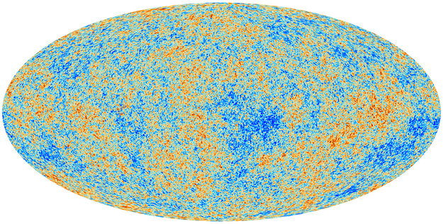
These are areas slightly colder or hotter than average and offer a picture of the spatial distribution of matter at the time when the CMB photons where able to free stream. So it is best for comparison to write our Boltzmann distribution perturbation as:

$f_{\gamma }={\displaystyle \frac{1}{e^{E/(T(t)+\mathrm{\Theta }(t,x,p))}-1}}\simeq {\displaystyle \frac{e^{E/T}}{{(e^{E/T}-1)}^2}}{\displaystyle \frac{\mathrm{\Theta }E}{T^2}}$ (12.18)

Unlike for galaxy surveys and other matter-related observables, the small perturbations stood small in the case of radiation so one can extend the wave-number analysis to smaller scales. Nonetheless it is not fully 3 dimensional information that we have on the CMB but bi-dimensional given by the direction one is looking at. So our Fourier decomposition is now discreet and given as

$\mathrm{\Theta }(x,p,\eta )=$ ${\displaystyle \sum _{l,m}}{a}_{l,m}(x,\eta )Y_{l,m}(\widehat{p})$ ${\displaystyle \int 𝑑{\mathrm{\Omega }}_{\widehat{p}}{Y}_{l,m}^{*}{Y}_{l^{\prime }{m}^{\prime }}}$ $={\delta }_{l{l}^{\prime }}{\delta }_{m{m}^{\prime }}$ (12.19)

where $\widehat{p}=p/|p|$ and now the two-field correlation reads:

$⟨⟨a_{lm}^{*}{a}_{l^{\prime }{m}^{\prime }}⟩⟩={\delta }_{l{l}^{\prime }}{\delta }_{m{m}^{\prime }}{C}_l$ (12.20)

with $m$-independent variance $C_l$. One can take the average then over different $m,m^{\prime }$ and the statistic limitation of the largest scales translates on the first few $l^{\prime }s$ having just $2l+1$ m terms. This in turn can be related to the power spectrum in the radiation field

$C_l={\displaystyle \int 𝑑{\mathrm{\Omega }}_{\widehat{p}}𝑑{\mathrm{\Omega }}_{{\widehat{p}}^{\prime }}^{\prime }{Y}_{lm}(\widehat{p})Y_{lm}^{*}({\widehat{p}}^{\prime })⟨⟨\mathrm{\Theta }(p)\mathrm{\Theta }(p^{\prime })⟩⟩}={\displaystyle \frac{2}{\pi }}{\displaystyle \int k^2𝑑k{P}_{\mathrm{\Theta }}(k)}$ (12.21)

Which can itself be to a matter power spectrum, see [5].

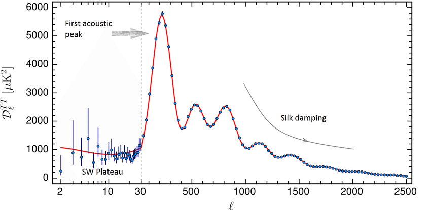
In addition there is more information on the CMB if one can measure the polarization of the photons, which is and objective experiments such as Bicep are pursuing.

12.3 Initial perturbations from inflation

The theory of inflation does more than growing the conformal time to solve the horizon problem; it provides the possible source of the initial perturbations. These are the seeds that through dynamics grow into the structure of everything we see today, although to explain ‘us’ inflation does not suffice but we need the matter over anti-matter asymmetry. The origin of these perturbation is in this context quantum fluctuations of the fields in inflation.

The process works approximately as this; the relevant fields and perturbations are those of the metric and the inflaton field. The inflaton field is driving inflation as some $\overline{\varphi }(t)$ to leading order which we refer to as the background field, just like there’s a background metric with $a(t)$. On top of this evolution quantum fluctuation of the field are allowed at the quantum level by the uncertainty principle, so we have $\varphi =\overline{\varphi }+\delta \varphi$

$⟨\mathrm{dS}|\varphi |\mathrm{dS}⟩$ $=0$ $⟨\mathrm{dS}|\varphi (\mathrm{k})\varphi ({\mathrm{k}}^{\prime })|\mathrm{dS}⟩$ $=P_{\varphi }(k){(2\pi )}^3{\delta }^3(k-k^{\prime })$ (12.22)

Where by $dS$ we mean the de-Sitter vacuum, that is an universe undergoing accelerated expansion. So to compute the power spectrum one should compute the two point correlator of the field in a background curved and dynamic space. This, although in an unfamiliar setting is a process which you have seen in QFT and here it can be simplified by using conformal time and some field redefinitions but it falls out of the range of these lectures, you can consult [5].

This spectrum of perturbations is however intrinsically quantum so they do not stick around, another key aspect of the background field is the acceleration of the scale factor. This means that scales $k$ in our spectrum will become larger than the horizon at some time. After this causal physics cannot operate and the perturbation stays frozen up until the inflationary phase stops and conformal time grows large enough so $\eta k\sim 1$. Borrowing results from the full computation the primordial power spectrum reads

$P_{\varphi }(k,\eta )$ $={(2\pi )}^3{k}^{3+n}$ $\mathrm{at}\mathit{\hspace{1em}}k\eta =1$ (12.23)

So the fluctuations are snatched away by causality and come back. The evolution is simple then for those perturbations which evolved the least, or those that re-entered horizon the latest. These are the largest scales which is why we say that inflation is probed on the small $l$ range of the angular power spectrum.

Finally we note that perturbations are produced in this way for all fields involved in inflation and this includes gravitons which we may hope to detect given that it’s proven possible for black hole and neutron mergers.

References

- [1] (2016) Planck 2015 results. XIII. Cosmological parameters. Astron. Astrophys. 594, pp. A13. External Links: 1502.01589, Document Cited by: §5.5.
- [2] (2020) Planck 2018 results. I. Overview and the cosmological legacy of Planck. Astron. Astrophys. 641, pp. A1. External Links: 1807.06205, Document Cited by: §1.1, §5.2, §5.3, §5.4, §5.6, §7.1.
- [3] (2020) First operation of the KATRIN experiment with tritium. Eur. Phys. J. C 80 (3), pp. 264. External Links: 1909.06069, Document Cited by: §5.2.
- [4] (2006) Dynamics of dark energy. Int. J. Mod. Phys. D 15, pp. 1753–1936. External Links: hep-th/0603057, Document Cited by: §5.6.
- [5] (2003) Modern cosmology. Academic Press, An Imprint of Elsevier, San Diego, California. External Links: ISBN 9780080511979 Cited by: 1st item, §12.2, §12.3.
- [6] (2015) An introduction to modern cosmology. Wiley, Chichester, West Sussex, United Kingdom. External Links: ISBN 1118690257 Cited by: 3rd item.
- [7] (2008) Cosmology. Oxford University Press, Oxford New York. External Links: ISBN 9780191523601 Cited by: 4th item.