
Let us now come back to our initial problem, the drop of milk in a cup of tea. We already know, in principle, what is going to happen in a simulation through random walkers from the previous one-dimensional example. We would like, however, to use the example now to discuss some aspects of non-equilibrium physics. In so doing we will focus on how a system starts at a non-equilibrium (namely the drop of milk as a "solid" block in the middle of the middle of the cup) and equilibrates over time (the milk being evenly distributed over the cup).
For simplicity, we assume a two-dimensional square cup with walls at x=±100 and y=±100, and the milk particles are forced to stay inside the cup. We also assume that the particles move on the sites of a square lattice, allowing for multiple occupancy per site - the results, in fact, would not change if only single occupancy was allowed. In the spirit of the lecture up to now, we allow the particles to undergo a random walk on the two-dimensional lattice, and in each time-step exactly one particle, chosen at random, is allowed to move by one unit either along the x or y direction. If this move carries the particle outside the cup (i.e. if, say,) x=101 after the random walk step, the cup's boundaries reflect it (in this example then x=99 after the random walk step). The results for 400 particles initialised as a compact drop in the middle of the cup undergoing a random walk as described after 0, 105, 106, and 107 time steps are shown below.
We could verify that the distribution of the particles as a function of time again follows the pattern of diffusion by, e.g. printing their density in a 3- dimensional plot, or by going to polar coordinates and checking the radial dimension only. However, here we would like to shift the focus and discuss how the results relate to the second law of thermodynamics, and the way in which such systems in statistical physics reach equilibrium. For this, an important quantity is the entropy. Roughly speaking, entropy is a measure of how ordered or disordered the system is. A perfectly ordered system has zero entropy, and entropy increases with the amount of disorder. Furthermore, statistical physics asserts as a theorem that the entropy of a closed system can only remain constant or increase over time.
This is something we could test with our little program simulating the milk-in-the-tea example. Initially, all milk particles are tightly packed in the middle of the cup, the system is highly ordered, and the entropy should be small. As time progresses the milk spreads out, disorder increases and the entropy increases with it. We can make this quantitative by explicitly calculating the entropy S of the system. Its definition in terms used in statistical physics reads
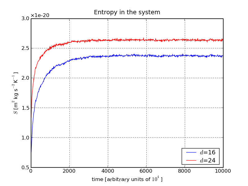
From the plot we see that, as time passes, the entropy rises until it reaches a more or less constant value, signalling the advent of an equilibrated state. At first sight it may be worrying that the entropy seems to depend on the number of cells/their cell-size, but in fact this is not relevant, since it is only the differences that matter. Apparently, once the effect of the finite cell-size has become unimportant, the two plots move in parallel.
This example shows how a closed system equilibrates. The particles spread to fill all states (here lattice sites) allowed to them uniformly, thus maximising the entropy. This is not built in the microscopic equations - our individual random walkers do not know anything about entropy. So why does this phenomenon occur? The answer sounds nearly banal: The system just spends time exploring all possible states, and as time progresses it will ultimately fill all states allowed to it with equal probability. There are, however, many more disordered than ordered states, so the system spends more time in the disordered states, thus equilibrating itself.
According to the ergodic hypothesis, all of the available states of a closed system in equilibrium will be occupied with equal probability - this is what we just mentioned. And, as already discussed, this is not a consequence of microscopic dynamics built in, e.g., Newton's laws. In fact, up to now, it was impossible to derive this hypothesis from any microscopic property or dynamics. Nevertheless, it is central to statistical physics and is in good agreement with all evidence. It is this principle, however, that ultimately leads to the fact that the entropy of a closed system can never decrease, which allows us to distinguish the past from the future when we see a movie.