A first numerical problem: Radioactive decays
← Previous
Construction of a working Python program: Code
This is the homework exercise. You will be given a skeleton code with
the task to expand it correspondingly. The skeleton code consists of three
files,
- A file called Radioactive.py,
which contains the physics problem. It is encapsulated in a
class.
A class is quite a high-level concept of something called
object-oriented (OO) programming, one of the newer paradigms. Here
it should suffice to say that classes act as some kind of "envelope"
around parameters and methods to modify them. In the case at hand,
the parameters contain, for instance, the time constant τ,
and the methods include, for example, the r.h.s. of the differential
equation
\[ \frac{\mathrm{d}N}{\mathrm{d}t}=-\frac{N}{\tau}\,\, . \]
In the homework, the students will supplement some of these methods.
In addition, this file also contains a __main__ method for input and
some plotting of results. The students are urged to look into it
as well (there's only a minor modification to be done there, the
input is half-life, but the class "Radioactive" needs the time
constant in its initialisation). This piece of the code incorporate
a number of python-specific commands and concepts. These allow for
comparably compact code, but are potentially hard to understand.
However, this is not so important for the basic understanding of the
numerical problem and its solution. The code presented here aims at
using the
"pylab"
-module
of python, which supports some very convenient features for plotting
etc..
- A file called Read_Type.py,
which contains a method to read a specific type (here a float number)
from the keyboard. As extra trick only numbers in a specified
range will be allowed - input from outside the range will lead to
an error message and program termination.
- A file called DEq_Solver.py,
which contains methods to solve first-order differential equations,
i.e. of the type
\[ \frac{\mathrm{d}\underline{x}}{\mathrm{d}t}=
\underline f(\vec x,t)\,\,, \]
or, in component form
\[ \frac{\mathrm{d}x_i}{\mathrm{d}t}=f_i(\{x_i\},t)\,\,. \]
Here, a class DEq_Solver is laid out which is meant to
incorporate different algorithms to solve such equations. All
these algorithms have in common that the solution is constructed
iteratively, as
\[\begin{eqnarray*}
\underline x_{i+1} &=& \underline x_i+\Delta\underline x =
x_i+f_i(\{x_i\},\,t)\Delta t\\
t_{i+1} &=& t_i + \Delta t\,,
\end{eqnarray*}\]
where, as indicated, $\Delta\underline x$ is determined by
$\underline f$, the r.h.s. of the differential equation. In the next
few homework exercises these algorithms will successively be built and
tested by the students.
The tricky issues are mainly concerned with the concept of a class,
and with the creation and handling of such objects. The students are
advised to take a closer look at the relevant chapters of the
Python online manual
or of the following
tutorial.
A number of issues related to programming are worth stressing:
- Structure:
Structured code typically is simpler to understand, to maintain, and
to debug. Try to make a point of using function definitions and,
eventually, multiple files to structure your program. Especially,
when you have pieces of your algorithm that are being used frequently
(like solving differential equations, etc.), clustering them into
individual functions and maybe even classes allows for recycling
successfully tested code and thus eases the validation of the
corresponding code and the construction of new ones.
Spaghetti-code may be simpler and quicker to produce, but typically
it is wasting time in the long run.
- Comments:
Use comments - maybe not as excessively as in the steering bit of
the code above, where some language explanations are entered, but
on a level that allows returning to the code later without having
to decipher its purpose all over again from scratch. As a rule of
thumb, try to make your programs "self-explaining".
- Clarity:
Try to program as clearly and transparently as possible. This may
be a nuisance while programmiong and a bit more costly in terms of
execution time of your code, but it is definitely worth it. During
code development it typically pays off in the end. It also allows for
collaborative coding.
The results of the program for dt=0.1 are shown in the figure below.
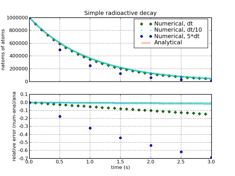 The error scales linearly with dt, as can be seen from running with
varying time step sizes dt, 5*dt and dt/10.
The error scales linearly with dt, as can be seen from running with
varying time step sizes dt, 5*dt and dt/10.
Next →
Frank Krauss and Daniel Maitre
Last modified: Tue Oct 3 14:43:58 BST 2017