Ising Model

←Previous

Phase transition a la MC

In this section we will discuss a first application of the Metropolis algorithm to the Ising model. For convenience we will think of the temperature, T, and the spin coupling constant, J, to be connected such that we give the temperature in units of J / k_B. In this lecture we will constrain ourselves to comparing the Monte Carlo results with those obtained from the mean field approximation. To this end we choose the external magnetic field to be zero, i.e. H=0, and we will consider the spontaneous magnetisation only. By now the construction of a Monte Carlo program implementing the Metropolis algorithm should not be too challenging, so here it should suffice to specify a few details that are to some extent subject to choices:

• Initialisation:
  In the example code we have implemented two options, namely either taking s_i=1 for all spins, or by choosing each of them at random to be either + or -1. In both cases we should allow a number of complete sweeps through the system to equilibrate it before we start taking averages.
• Boundary conditions:
  In the ideal case, we would like to consider large lattices. In reality, however, this is not always possible, with the effect that more than often a sizable fraction of spins finds itself at the edges. This can lead to pronounced effects, known as finite-size effects. Of course, such effects also appear in real systems, but typically the lattices in, say a block of iron, contain a macroscopically large number of sites (i.e. atoms), of the order of 10²³. This obviously is beyond the realm of current computers. Therefore it is important in the simulations to minimise the finite-size effects. The arguably most prominent way of doing this is to use periodic boundary conditions. They work as follows: If a spin is on the edge, the spin at the opposite edge is taken as its nearest neighbour, such that the system does not have any spins on the edge. In terms of geometry, our two-dimensional lattice would have something like a doughnut-shape. Nevertheless, it should be stressed that a 5⊗5 lattice with periodic boundary conditions will not behave the same way as a much larger system. For any L⊗L system the maximal distance between two spins cannot be larger than L/√2 lattice spacings, this will become important in the next lecture when we consider correlation lengths etc..
• Sweeping through the lattice:
  In our example program we have implemented two ways of sweeping through the lattice, one by selecting the spin to potentially flip by random, the other by systematically going through the lattice, line by line, spin by spin.

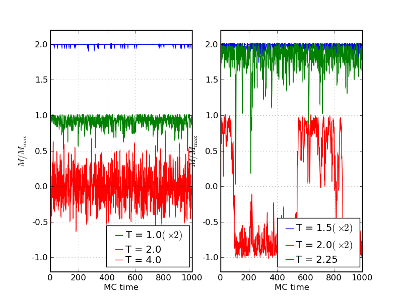
For our simulations we run over a 10⊗10 lattice with periodic boundary conditions, where we initialised all spins to point into the same plus direction initially, and we systematically sweep through the lattice. Although we could, in principle, work out a way to relate the Monte Carlo time expressed by sweeps with some real time, we will use a notion; each sweep testing, on average, every spin in the lattice is used as the basic unit of time. In the plot below we exhibit how the system behaves at various different temperatures.

We clearly see that at low temperatures, the system is fairly stable with only small fluctuations, and the magnetisation is more or less equal to 1. Already at T=2, the Boltzmann factor favours a spin flip out of phase with a probability of around 10%, and consequently the average magnetisation falls to about 0.9. At even larger temperatures, around or larger than T=4 the spins are more or less disordered, and the system fluctuates around M=0, the paramagnetic state. This implies that the value of T_c=4 found for the critical temperature in the mean field approximation is not reproduced by the Monte Carlo method. A careful analysis will show that this holds true also in the limit of infinitely large lattices. Instead, it seems as if the phase transition occurs at temperatures around T=2.25. There (see right panel), the system seems to be fairly stable for quite some time before it "jumps" into another magnetisation state. It also becomes apparent that the size of the fluctuations increases with temperature. This is important for various reasons. First of all, the fluctuations contribute to the thermal average, and larger fluctuations will move, for instance, the magnetisation away from M=0 as temperature increases, and with it the size of the fluctuations. In addition, we will see in the next lecture, how the fluctuation-dissipation relation can be used to deduce physical observables from their size. Finally, and probably most importantly, their enhancement signals that a second-order phase transition, also known as critical point is approached. At this critical point, systems are extremely sensitive to small perturbations, and its properties change rapidly in response to changes in temperature, magnetic field, etc.. We will learn that the fluctuations are deeply connected to such singular behaviour. When warming up the system to temperatures around the critical point, the fluctuations become larger, until they are so large that the magnetisation of the entire system changes sign. In our example this happens at T=2.25 - we know already that this is close to the true critical point T_c=2.27.

We can check this finding by considering the magnetisation M as a function of the temperature T. We can do this in the simulations by sweeping initialising the lattice several times at each temperature, and sweeping through the lattice. After some number of initial sweeps, ensuring some first equilibration, we can take the magnetisation after each complete sweep. Averaging over the results will then yield the thermal average M(T), shown in the plot below.

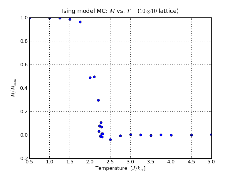
Looking back to the time series at different temperatures it becomes apparent that it is mandatory to allow the system enough steps to reach equilibrium. The time, i.e. the number of sweeps, necessary for this is strongly temperature-dependent and on how far the initial state is from the true equilibrium. At temperatures away from the critical point, this time is indeed very short (as can be seen in the plot above), but while approaching the critical point, the equilibration time increases, until it diverges at the critical point. This is known as critical slow down, and it prevents us from having very good results in the plot above. As can be seen there, the magnetisation has a substantial scatter around T_c. From the plot above we see that M drops precipitously to zero around the critical temperature. To improve the scattered results we could try to employ more sweeps through the lattice, since statistical errors reduce roughly like √N_steps with the number of time steps taken. Secondly, we could study larger lattices and try to extrapolate to infinite lattice size. We leave this to the interested reader, who may want to modify the code to do that.

In any case, it is interesting to compare, at this point, the results of the Monte Carlo simulation with the results from the mean field approximation. We find that the critical temperature differs by a factor of roughly two, and we could read off that the critical is different from 1/2, the mean field result. These finding are in agreement with more precise analytical calculations, verifying the Monte Carlo results. In the next lecture we will examine these differences a bit closer, by employing more observables.

Next→