Mean field theory is an extremely powerful approximation to problems with many interacting particles, including our Ising model. We will introduce it very briefly, strictly in the context of our problem. We will use it to deduce some properties of the Ising model, in particular the phase transition it experiences. However powerful at first sight, this method is far from being overly accurate, it lacks quantitative precision. So this discussion here will rather aim at a qualitative understanding, and we will revisit most of the issues in the context of our simulation.
We have seen that magnetisation in the Ising model is closely related to the alignment of the spins, and therefore to their thermal average. It is useful to think of this as a time average (for instance during the measurement procedure) of the system in thermal equilibrium with the heat bath. Such an average obviously "averages out" the effect of the individual spin flips, moving the system from one micro-state to another. For an infinitely large system, all spins then will have the same average alignment. To see this, notice that all spins are equivalent, since they all interact with their nearest neighbours - in the case we will consider most of the time, we will have a square lattice in 2 dimensions, and therefore j=4 nearest neighbours - and all are infinitely far away from the boundaries. So, no spin is special, and all must have the same average properties. The total magnetisation at temperature T therefore reads
While in the first term we summed over all spins i, in the second
expression we used the fact that all spins have the same average properties, and
we picked one, also denoted by i. To compensate for the sum, we multiplied
with the total number of spins. Therefore, in this approach, we are done once we
manage to calculate the average behaviour of one spin. This, however, is tricky,
because again all the micro-state probabilities etc. would kick in. Therefore,
let us try something different.
The trick is to add a magnetic field, H, which also points along the
positive or negative z-axis. The energy function then reads
Here, μ is the magnetic moment of each spin. This additional field
will lead to the spins being more likely to orient themselves in parallel to it,
since this lowers the energy of the overall system.
Let us, for the moment, consider one spin si in the external
field alone. Then the only energy involved is the external field, H. The
two possible states si=±1 have energies
and the probabilities of finding the system in either of the two states are given by
where the normalisation constant follows from requiring that both probabilities add up to unity:
The thermal average of the single spin therefore is
This indeed is the exact behaviour of a single spin in an external
magnetic field. We will use this now as the basis for an approximate solution for
a system of N interacting spins.
The idea becomes apparent when we rewrite the energy function in the suggestive
form
and replace the term in the bracket with an effective magnetic field
Here the sum still extends over the nearest neighbours of spin si. This shows that the effect of the other spins on any individual spin si takes the form of a magnetic field, identical to the effect an external field would have. And now comes the approximation: Rather than explicitly calculating the neighbouring spins and using them to determine this effective magnetic field, the mean field approximation replaces them with their averages. Setting the external field to 0, the mean field approximation to the effective magnetic field reads
Again, j is the number of nearest neighbour sites. Plugging this into the equation determining the average of the spins above yields an implicit equation for this average, namely
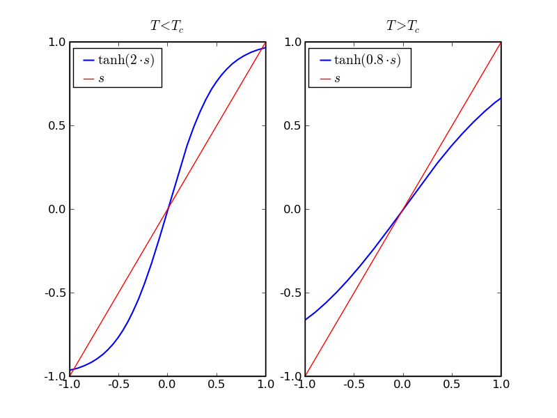
This equation cannot be solved analytically, except in the limit when the spin- average < s > is small. Therefore we would have to resort to the root-finding methods we discussed a few lectures ago. To illustrate the nature of the problem, the schematic plot below shows two different parameter choices:
There are clearly two regimes, characterised by different values of the temperature, if J and the lattice geometry are fixed. In a regime of low temperature, the implicit equation for the average spin has three solutions, while at high temperatures there is only one solution. This solution of zero average spin implies zero magnetisation: The system is in a paramagnetic phase. At low temperatures, when there are two additional solutions at ± s0, there are two phases with non-zero and opposite magnetisation. These are the ferromagnetic phases. The question now is, which of the multiple solutions is the one the system prefers. To answer this, it is useful to consider the free energy of the system for the various solutions. It turns out that the ferromagnetic solutions have the smaller free energy, implying that the system would find itself in either of the ferromagnetic phases at low temperatures. The exact magnetisation, i.e. whether the system is in the +s0 or in the -s0, is distributed equally. This symmetry (or degeneracy) is lifted by switching on the external magnetisation. However, these findings immediately translate into the existence of a phase transition in the Ising model, from the para- to the ferromagnetic phase, occurring at a critical temperature Tc. For the numerical determination of the exact solutions ± s0, given by the equation
we will use parameters such that Tc=4.
In the plot below we show the positive branch of the solution from the mean field approximation. Since the magnetisation is proportional to the average of s, there is spontaneous magnetisation of maximal size Mmax = N at T=0, which vanishes with rising temperatures. When the critical temperature Tc=4 is approached, the magnetisation's slope changes discontinuously, signalling a second-order phase transition.
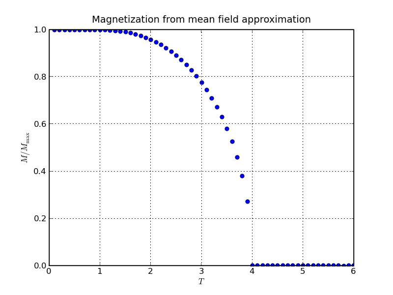
This phase transition is similar to the one encountered in the case of percolation before. While there, the occurrence of percolating clusters or their occupancy served as order parameter in the case of the Ising model it is the magnetisation, whose abrupt change signals the phase transition: The order parameter indicates the phase the system is in. The results from the plot above suggest that while M vanishes in a singular manner as the temperature becomes critical, dM/dT becomes extremely large around Tc. The form of this singularity can be obtained by expanding around small average spin, i.e for < s > → 0. Using the Taylor expansion of tanh(x) around small x,
yields
and therefore, as non-trivial solution,
From this we read off the critical temperature, Tc=(j J)/(kBT) and the critical exponent, β=1/2.
Again, as in the case of percolation, we find a power law describing the behaviour of important properties. It should be stressed, however, that although the mean field approximation employed here yields the correct behaviour on the qualitative level, the numerical results are by no means correct. In fact, for a square lattice in two dimensions, with 4 neighbouring sites, an exact calculation yields Tc=2/ln(1+√2), roughly 2.27, and β=1/8!